1 CENTRO DE NEUROCIENCIAS DE CUBA SUBDIRECCIÓN DE NEUROINFORMÁTICA LABORATORIO DE NEUROIMÁGENES CARACTERIZACIÓN DE LA CONECTIVIDAD ANATÓMICA CEREBRAL A PARTIR DE LAS NEUROIMÁGENES DE LA DIFUSIÓN Y LA TEORÍA DE GRAFOS Trabajo de Tesis para optar por el grado de Doctor en Ciencias de la Salud Yasser Iturria Medina Ciudad de la Habana 2012
Transcript
1
CENTRO DE NEUROCIENCIAS DE CUBA
SUBDIRECCIÓN DE NEUROINFORMÁTICA
LABORATORIO DE NEUROIMÁGENES
CARACTERIZACIÓN DE LA CONECTIVIDAD
ANATÓMICA CEREBRAL A PARTIR DE LAS
NEUROIMÁGENES DE LA DIFUSIÓN Y LA
TEORÍA DE GRAFOS
Trabajo de Tesis para optar por el grado
de Doctor en Ciencias de la Salud
Yasser Iturria Medina
Ciudad de la Habana
2012
2
CENTRO DE NEUROCIENCIAS DE CUBA
SUBDIRECCIÓN DE NEUROINFORMÁTICA
LABORATORIO DE NEUROIMÁGENES
CARACTERIZACIÓN DE LA CONECTIVIDAD
ANATÓMICA CEREBRAL A PARTIR DE LAS
NEUROIMÁGENES DE LA DIFUSIÓN Y LA
TEORÍA DE GRAFOS
Trabajo de Tesis para optar por el grado
de Doctor en Ciencias de la Salud
Por
Autor: MSc. Yasser Iturria Medina
Tutor: DrC. Nelson Trujillo Barreto
Ciudad de La Habana
2012
3
AGRADECIMIENTOS
Empecé a trabajar en temas de tractografía con Pedro A. Valdés Hernández,
hace unos ocho años, cuando este aspiraba a un método nuevo para dar peso a
las conexiones entre diferentes regiones cerebrales. A este esfuerzo pronto se
sumó Erick J. Canales, dedicado más a la caracterización de la anisotropía
intravoxel, junto a Lester Melie García y Yasser Alemán Gómez, pero siempre
dispuesto a aportar ideas valiosas al análisis de la conectividad anatómica. La
caracterización de las redes de conectividad comenzó, no mucho después, con
Roberto Carlos Sotero, quien también dio aplicación a los métodos que iban
surgiendo en modelos de actividad neural que desarrolló junto a Nelson Trujillo.
Esos fueron los principios: todos inspirados a la vez en la bibliografía que surgía.
A todos agradezco.
Cuando intenté dar otras aplicaciones a los métodos creados, Alejandro Pérez
Fernández contribuyó a mejorar mis preguntas, muchas de las ideas actuales y
planes futuros, sobre todo aquellos relacionados al estudio de patologías
específicas, provienen de esa colaboración. También le debo cierta valiosa
intervención para revisar esta tesis, labor a la que se han sumado, para mi
suerte, María Antonieta Bobes, Ramón Martínez Cansino, Marlis Ontivero
Ortega, Lester Melie García, Nelson Trujillo Barreto, Calixto Machado Curbelo y
José Miguel Bornot.
Espero haber aprovechado las sugerencias de todos, y más aún, que el texto
final cumpla por fin con sus expectativas.
4
SÍNTESIS
Las neuroimágenes de la difusión permiten reconstruir las trayectorias que
presentan las fibras nerviosas de la materia blanca. Sin embargo, las
metodologías asociadas presentan limitaciones y carecen de una formulación
directa para caracterizar las conexiones anatómicas entre estructuras de la
materia gris. En la presente tesis se aborda el problema de la caracterización de
las conexiones anatómicas cerebrales basándonos en la información contenida
en las neuroimágenes de la difusión y en la capacidad de la teoría de grafos
para modelar matemáticamente relaciones cualesquiera entre objetos. En un
primer paso, se combinan elementos de la teoría de grafos y de las
neuroimágenes de la difusión para reconstruir y caracterizar las trayectorias de
las fibras nerviosas entre diferentes regiones de interés. En un segundo paso, la
metodología anterior es utilizada para reconstruir las redes anatómicas
cerebrales de un grupo de humanos saludables, y luego se caracterizan estas
redes empleando un conjunto de medidas topológicas que evalúan sus
capacidades para lidiar con el flujo de información neural. En un tercer paso, se
comparan los dos hemisferios cerebrales (en humanos saludables y un primate
no-humano) según las características topológicas de sus correspondientes
subredes anatómicas. En el cuarto y último paso, se propone analizar la
topología de la red anatómica cerebral para discriminar condiciones cerebrales
anómalas, y se analiza el caso de un modelo animal relevante para el estudio de
las enfermedades desmilienizantes. Todos los métodos que se proponen han
sido validados en datos simulados y reales, y los resultados han sido publicados
El advenimiento de las modernas técnicas de neuroimágenes ha generado una
verdadera revolución en la comprensión del complejo sistema nervioso humano.
La Tomografía Axial Computadorizada (TAC), la Tomografía por Emisión de
Positrones (PET) y la Resonancia Magnética Nuclear (RMN), son algunos
ejemplos de técnicas de relativa reciente aparición, que permean incluso el
vocabulario común y la vida cotidiana. Estas técnicas posibilitan como nunca
antes el acceso en forma de imágenes a la estructura del cerebro. Y no sólo eso,
permiten además observar su funcionamiento en el tiempo: la progresiva
activación de diferentes áreas cerebrales en la medida que una persona realiza
determinada actividad mental. En general, gracias a ellas el estudio y la
comprensión del cerebro ha tenido un desarrollo vertiginoso, convirtiendo en
obsoleta aquella visión de "caja negra" que antes teníamos sobre este. Un rol
exclusivo en estos avances lo tiene la RMN, técnica que cuenta con la enorme
ventaja de ser no-invasiva. Las imágenes así obtenidas se basan en la
cuantificación de las propiedades magnéticas de los diferentes tejidos,
guardando distancia del proceso físico de la radiación y sus indeseables
consecuencias, algo que sí está presente en las técnicas de TAC y PET. En
parte por eso, su uso es muy amplio, sea en la clínica o en la investigación. Pero
también porque a través de ella podemos desde explorar la integridad tisular,
hasta inferir las zonas que se activan ante determinado proceso cognitivo,
pasando por la posibilidad que brindan para determinar cómo están conectadas
anatómica/funcionalmente unas y otras zonas del cerebro. Se podría afirmar que
la información que esta técnica nos ofrece es tan rica y variada, que por ahora
las limitaciones a su uso no son otras que las que imponga nuestro ingenio en la
definición de nuevas metodologías para el análisis e interpretación del enorme
caudal de datos que nos ofrece la RMN.
En este sentido, las neuroimágenes de la difusión han resultado ser una de las
modalidades de más sorprendente desarrollo entre las técnicas de RMN.
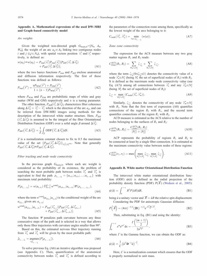
8
Básicamente, las neuroimágenes de la difusión, también llamadas imágenes de
resonancia magnética nuclear ponderadas en difusión, reflejan cómo ocurre el
movimiento caótico de las moléculas de agua embebidas entre los diferentes
tejidos cerebrales (Basser y col., 1994; LeBihan D. y col., 2001; LeBihan, 1995).
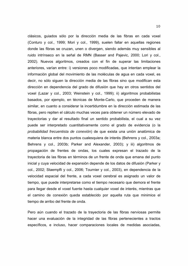
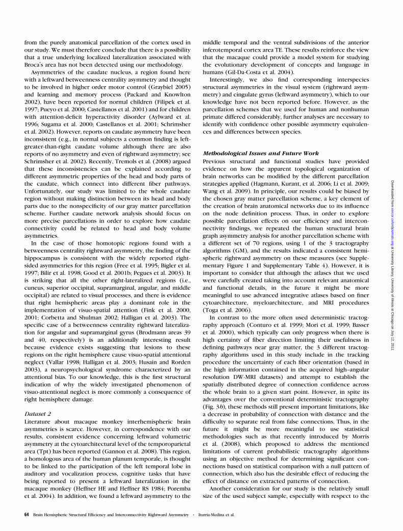
Como se ilustra en la Figura 1a, el proceso de difusión del agua en la materia
blanca se encuentra relacionado a la organización estructural de las fibras
nerviosas: las moléculas fluyen con mayor facilidad en la dirección paralela a las
fibras (donde se considera que la difusión es libre, pues no existen barreras) que
en la dirección perpendicular (donde la difusión es restringida, pues las
moléculas chocan con las paredes de los axones). Si dividiéramos todo nuestro
cerebro en pequeños volúmenes cúbicos iguales (a los que suele llamárseles
voxeles), y adquiriéramos una imagen típica de difusión, obtendríamos para
cada voxel un valor de intensidad en la imagen: cuando el valor es bajo (pixel
oscuro en la imagen), puede decirse que en este voxel hay mucha difusión en
una dirección dada, y cuando el valor de intensidad es alto (pixel brillante en la
imagen), se dice que ocurre poca difusión en la dirección observada. Esto
permite investigar en qué direcciones específicas, de cada voxel, se mueven
más las moléculas de agua, que como ya sabemos están “obligadas” a moverse
en sentido paralelo a las fibras, por lo que de manera indirecta finalmente se
asume que las fibras nerviosas en cada voxel están orientadas en aquellas
direcciones en que más se movieron las moléculas de agua (Basser y col., 1994;
Basser y col., 2000; Basser, 2002). La Figura 1b ilustra este proceso: en cada
uno de los pequeños volúmenes en que hemos dividido el cerebro se obtiene
una posible direccionalidad de las fibras contenidas. Una aplicación básica es
emplear esta información direccional para seguir, de punto en punto (voxel a
xoxel), la trayectoria de las fibras nerviosas al conectar las diferentes estructuras
cerebrales (Ito y col., 2002; Mori y col., 1999), tal como se ilustra en la Figura 1c.
9
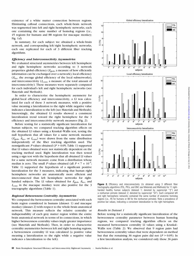
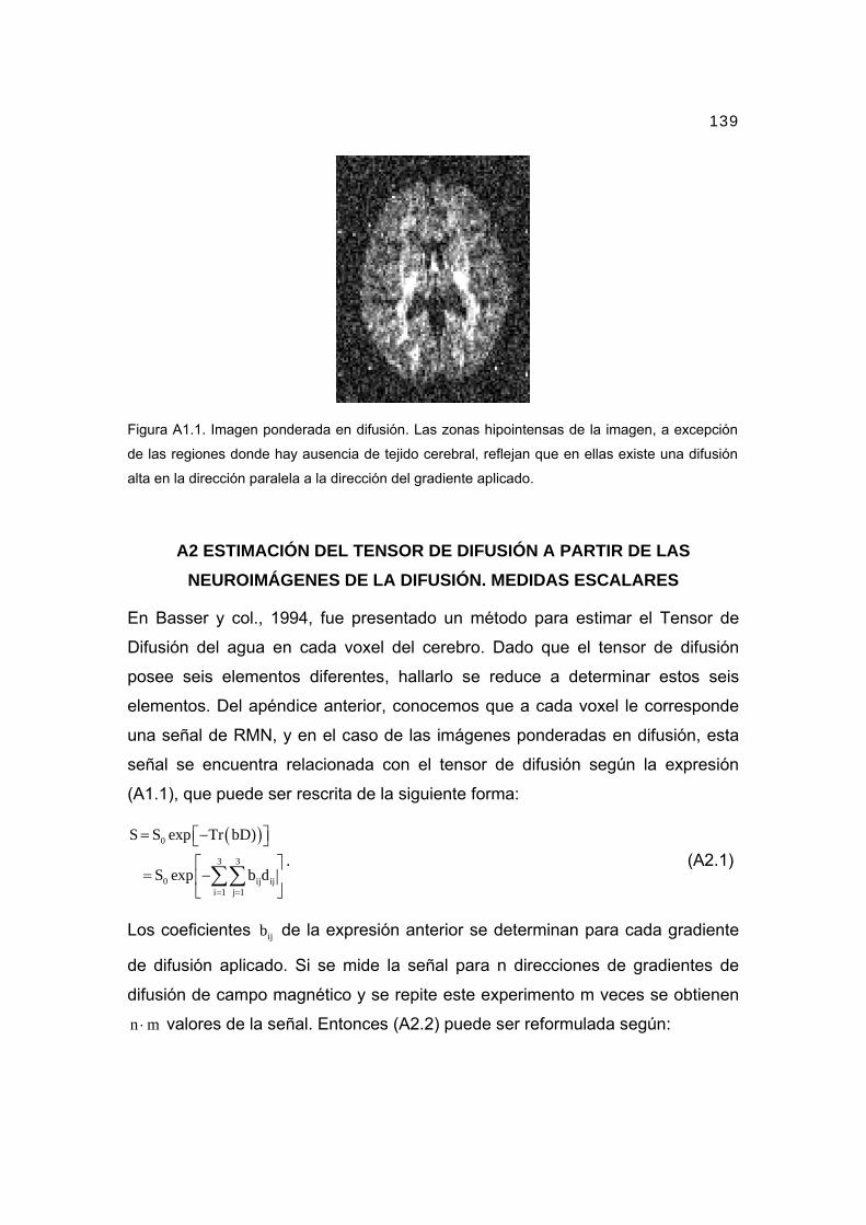
Figura 1. Del movimiento de las moléculas de agua a la reconstrucción de la trayectoria de las
fibras nerviosas. a) Representación hipotética del movimiento de moléculas de agua (líneas
blancas quebradas) alrededor de tres axones paralelos. b) Plano coronal del cerebro en el cual
se presenta la dirección media de las fibras nerviosas en cada voxel. c) Trayectorias de fibras
nerviosas estimadas a través de todo el cerebro luego de seguir de punto en punto la dirección
media de las fibras obtenidas en cada voxel (Mori y col., 1999). En b) y c), el color de cada
segmento o trayectoria se asignó de acuerdo al código RGB, según el cual cada vector toma un
color que corresponde con su dirección. Por ejemplo, el color rojo indica que la orientación media
de las fibras nerviosas es en la dirección medio-lateral, mientras el color verde corresponde a
aquellas fibras orientadas en la dirección antero-posterior, y el color azul a las fibras orientadas
en la dirección supero-inferior.
La obtención de las trayectorias que presentan las fibras nerviosas al conectar
las diferentes estructuras que procesan la información neural, ha permitido
profundizar por primera vez en la caracterización de la anatomía cerebral y en el
entendimiento de la integración funcional del cerebro humano (Behrens y col.,
2003a; Koch y col., 2002; LeBihan D. y col., 2001; Ramnani y col., 2004; Sotero
y col., 2007; Sporns y col., 2005). Y todo esto es posible por primera vez in vivo,
con el consiguiente impacto sobre el asesoramiento del estado de conectividad
cerebral puntual de determinado ser vivo. Sin embargo, el punto álgido del tema
lo constituyen aquellos algoritmos que permiten pasar de la estimación de la
posible direccionalidad de las fibras en cada voxel (figura 1b) a la estimación de
los tractos que conectan las regiones (figura 1c). Existe un consenso cada vez
mayor sobre las múltiples limitaciones que poseen los algoritmos actuales de
reconstrucción de trayectorias de fibras nerviosas. En particular los algoritmos
10
clásicos, guiados sólo por la dirección media de las fibras en cada voxel
(Conturo y col., 1999; Mori y col., 1999), suelen fallar en aquellas regiones
donde las fibras se cruzan, unen o divergen, siendo además muy sensibles al
ruido intrínseco en la señal de RMN (Basser and Pajevic, 2000; Lori y col.,
2002). Nuevos algoritmos, creados con el fin de superar las limitaciones
anteriores, varían entre: i) versiones poco modificadas, que intentan emplear la
información global del movimiento de las moléculas de agua en cada voxel, es
decir, no sólo siguen la dirección media de las fibras sino que modifican esta
dirección en dependencia del grado de difusión que hay en otros sentidos del
voxel (Lazar y col., 2003; Weinstein y col., 1999); ii) algoritmos probabilistas
basados, por ejemplo, en técnicas de Monte-Carlo, que proceden de manera
similar, en cuanto a considerar la incertidumbre en la dirección estimada de las
fibras, pero repiten el cálculo muchas veces para obtener un número elevado de
trayectorias y dar al resultado final un sentido probabilista, el cual a su vez
puede ser interpretado cuantitativamente como el grado de evidencia (o la
probabilidad frecuentista de conexión) de que exista una unión anatómica de
materia blanca entre dos puntos cualesquiera de interés (Behrens y col., 2003a;
Behrens y col., 2003b; Parker and Alexander, 2003); y iii) algoritmos de
propagación de frentes de ondas, los cuales expresan el trazado de la
trayectoria de las fibras en términos de un frente de onda que emana del punto
inicial y cuya velocidad de expansión depende de los datos de difusión (Parker y
col., 2002; Staempfli y col., 2006; Tournier y col., 2003), en dependencia de la
velocidad espacial del frente, a cada voxel cerebral es asignado un valor de
tiempo, que puede interpretarse como el tiempo necesario que demora el frente
para llegar desde el voxel fuente hasta cualquier voxel de interés, mientras que
el camino de conexión queda establecido por aquella ruta que minimice el
tiempo de arribo del frente de onda.
Pero aún cuando el trazado de la trayectoria de las fibras nerviosas permite
hacer una evaluación de la integridad de las fibras pertenecientes a tractos
específicos, e incluso, hacer comparaciones locales de medidas asociadas,
11
nuestra comprensión de la conectividad anatómica cerebral queda restringida a
la comprensión de sus características anatómicas locales. Consideramos
entonces que los estudios en el marco de las neuroimágenes de la difusión
podrían ir mucho más allá y emplear las trayectorias estimadas de las fibras para
caracterizar cuantitativamente las conexiones anatómicas entre diferentes
regiones de materia gris, permitiendo no sólo describir conexiones específicas
sino también evaluar las relaciones entre ellas y sus potencialidades para
gestionar e integrar el flujo de información neural. Esto permitiría
consecuentemente evaluar daños provocados por aquellos desórdenes o
patologías cerebrales que alteran las conexiones nerviosas entre los diferentes
centros de procesamiento de la actividad neural.
En particular, el uso de la teoría de grafos, cuyo surgimiento se inspira en las
soluciones que en el siglo XVI Euler brindara al problema de encontrar el camino
optimo para cruzar siete puentes de un río, permitiría la modelación de las
conexiones cerebrales desde el punto de vista de nodos y arcos que
representen todas las posibles conexiones entre las diferentes regiones
anatómicas y funcionales. Este tipo de enfoque, intuitivamente muy simple pues
condensa el complejo sistema de conexiones cerebrales a sólo un conjunto de
puntos y líneas en el espacio, permitiría además caracterizar el patrón de las
conexiones según un compendio de herramientas y medidas topológicas
físicamente interpretables que han sido desarrolladas en las últimas décadas,
bajo el albor de la teoría de grafos, para el análisis cuantitativo de las redes
sociales y biológicas (Albert y col., 1999; Bassett and Bullmore, 2006a; Milos y
col., 2002; Salvador y col., 2005a).
12
1.1. PROBLEMA CIENTÍFICO
Las metodologías actuales basadas en técnicas de las neuroimágenes de la
difusión no permiten de forma directa: cuantificar las conexiones anatómicas
entre regiones cerebrales de interés, caracterizar la red estructural asociada,
según su capacidad para lidiar con el flujo de información neural, y evaluar las
afectaciones estructurales provocadas por condiciones patológicas.
13
1.2. HIPÓTESIS
La combinación de las técnicas basadas en neuroimágenes de la difusión con
elementos de la teoría de grafos permite la estimación de las conexiones
anatómicas cerebrales, la caracterización de la red estructural asociada, según
su capacidad para lidiar con el flujo de información neural, y la evaluación de las
afectaciones provocadas por condiciones patológicas.
14
1.3. OBJETIVO GENERAL
Desarrollar una metodología, sobre el marco de las técnicas basadas en
neuroimágenes de la difusión y la teoría de grafos, que permita estimar las
conexiones anatómicas cerebrales, caracterizar la red estructural asociada,
según su capacidad para lidiar con el flujo de información neural, y evaluar las
afectaciones provocadas por condiciones patológicas.
1.3.1. OBJETIVOS ESPECÍFICOS
1. Evaluar la conectividad anatómica entre diferentes regiones cerebrales a
partir de la reconstrucción de las trayectorias de las fibras nerviosas.
2. Caracterizar topológicamente la red anatómica cerebral de humanos
típicos o sanos.
3. Estimar si existen diferencias interhemisféricas en las redes anatómicas
en cuanto a la eficiencia y optimización estructural para lidiar con el flujo
de información neural.
4. Evaluar la capacidad de las propiedades topológicas de la red anatómica
cerebral para discriminar automáticamente una condición cerebral
patológica.
1.3.2. TAREAS A CUMPLIR SEGÚN LOS OBJETIVOS ESPECÍFICOS
Relacionadas al objetivo 1:
1.1 Desarrollar un algoritmo que permita trazar la trayectoria de las fibras
nerviosas entre diferentes estructuras cerebrales de interés.
1.2 Explorar en datos simulados y experimentales el comportamiento del
algoritmo anterior, así como comparar su comportamiento con el de otros
algoritmos propuestos anteriormente en la literatura.
15
1.3 Definir medidas geométricas para cuantificar las conexiones anatómicas
entre diferentes estructuras de la materia gris, que pueden ser
delimitadas de acuerdo a criterios histológicos, citoarquitectónicos o
funcionales, a través de segmentaciones manuales, automáticas o
semiautomáticas.
1.4 Explorar en datos simulados el comportamiento de las medidas definidas
anteriormente para evaluar la conectividad entre estructuras de la
materia gris, así como evaluar si son capaces de reflejar pérdidas
hipotéticas de la integridad en la materia blanca.
1.5 Aplicar los métodos anteriores para calcular mapas de conectividad
anatómica entre diferentes estructuras de la materia gris
correspondientes a varios sujetos humanos sanos.
Relacionadas al objetivo 2:
2.1 Reconstruir la red estructural del cerebro humano sano a partir de los
mapas de conectividad anatómica obtenidos entre las diferentes
estructuras de la materia gris.
2.2 Evaluar medidas topológicas que describan las características
intrínsecas de la red estructural del cerebro humano sano, teniendo en
cuenta la disponibilidad local y global para el manejo e integración del
flujo de información neural.
Relacionadas al objetivo 3:
3.1 Reconstruir la red estructural de los hemisferios izquierdo y derecho
(para sujetos humanos y un primate no-humano) a partir de los mapas de
conectividad anatómica obtenidos entre las diferentes estructuras de la
materia gris, según diferentes métodos de trazado de las trayectorias de
fibras nerviosas.
3.2 Evaluar e interpretar, para cada especie, medidas topológicas que
describan las semejanzas y diferencias entre sus hemisferios cerebrales,
16
teniendo en cuenta la disponibilidad local y global para el manejo e
integración del flujo de información neural.
Relacionadas al objetivo 4:
4.1 Reconstruir la red estructural del cerebro de ratones portadores de una
mutación que provoca una sintomatología equivalente a la esclerosis
múltiple en humanos (a los que nos referiremos como ratones
temblorosos, del inglés Shiverers) y controles de igual rango de edad, a
partir de los mapas de conectividad anatómica obtenidos entre las
diferentes estructuras de la materia gris, según diferentes métodos de
trazado de las trayectorias de fibras nerviosas.
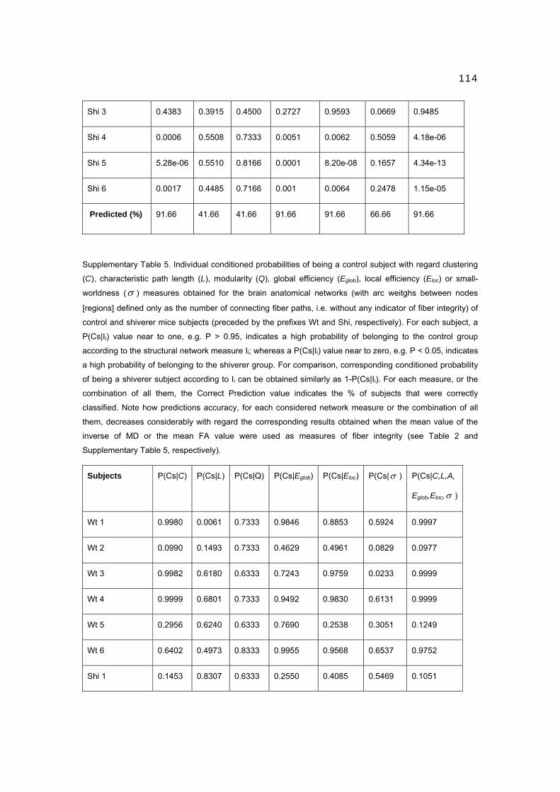
4.2 Clasificar, según las características topológicas de las redes anatómicas
individuales, a cada ratón de la muestra como sujeto patológico o sujeto
control, obteniendo para ello un valor de probabilidad de pertenecer a un
grupo u otro como índice individual de clasificación anatómica.
17
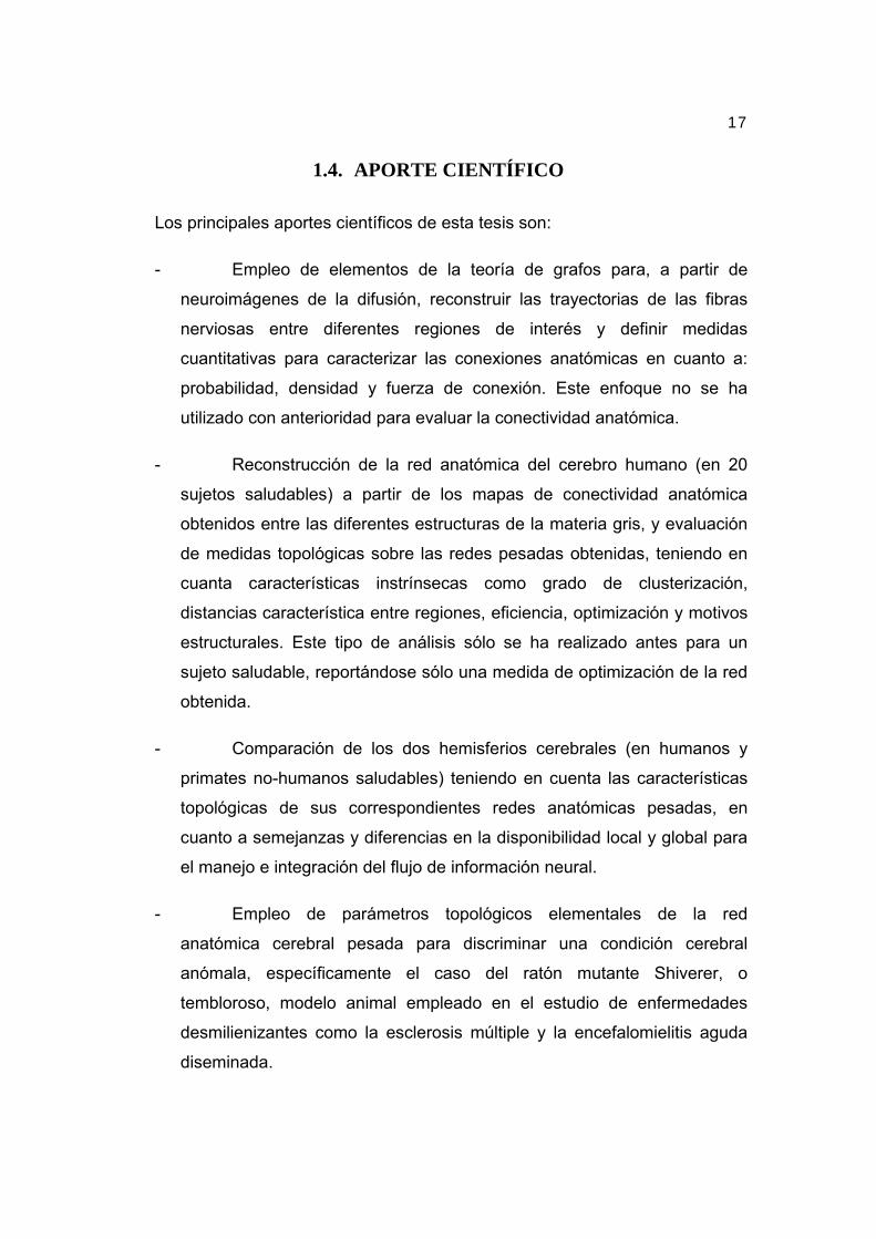
1.4. APORTE CIENTÍFICO
Los principales aportes científicos de esta tesis son:
- Empleo de elementos de la teoría de grafos para, a partir de
neuroimágenes de la difusión, reconstruir las trayectorias de las fibras
nerviosas entre diferentes regiones de interés y definir medidas
cuantitativas para caracterizar las conexiones anatómicas en cuanto a:
probabilidad, densidad y fuerza de conexión. Este enfoque no se ha
utilizado con anterioridad para evaluar la conectividad anatómica.
- Reconstrucción de la red anatómica del cerebro humano (en 20
sujetos saludables) a partir de los mapas de conectividad anatómica
obtenidos entre las diferentes estructuras de la materia gris, y evaluación
de medidas topológicas sobre las redes pesadas obtenidas, teniendo en
cuanta características instrínsecas como grado de clusterización,
distancias característica entre regiones, eficiencia, optimización y motivos
estructurales. Este tipo de análisis sólo se ha realizado antes para un
sujeto saludable, reportándose sólo una medida de optimización de la red
obtenida.
- Comparación de los dos hemisferios cerebrales (en humanos y
primates no-humanos saludables) teniendo en cuenta las características
topológicas de sus correspondientes redes anatómicas pesadas, en
cuanto a semejanzas y diferencias en la disponibilidad local y global para
el manejo e integración del flujo de información neural.
- Empleo de parámetros topológicos elementales de la red
anatómica cerebral pesada para discriminar una condición cerebral
anómala, específicamente el caso del ratón mutante Shiverer, o
tembloroso, modelo animal empleado en el estudio de enfermedades
desmilienizantes como la esclerosis múltiple y la encefalomielitis aguda
diseminada.
18
2. DESCRIPCIÓN DE LOS ARTÍCULOS
2.1. EVALUACIÓN DE LA CONECTIVIDAD ANATÓMICA ENTRE
DIFERENTES REGIONES CEREBRALES A PARTIR DE LA
RECONSTRUCCIÓN DE LAS TRAYECTORIAS DE FIBRAS
NERVIOSAS
Alrededor de un 60 % del volumen cerebral está compuesto por agua que
difunde continuamente, debido al movimiento caótico de sus moléculas, entre los
diferentes tejidos cerebrales. Pero la movilidad de estas moléculas de agua no
siempre es la misma en todas las direcciones, depende de las características
locales de los tejidos, que representan en sí mismos barreras estructurales y
permiten en menor o mayor medida los procesos difusivos. Por ejemplo, el
movimiento de las moléculas de agua en el líquido cefalorraquídeo1 tiende a ser
igual en todas las direcciones espaciales, o isotrópico, dado que no existen
barreras que interfieran ante la movilidad de las moléculas; en cambio, el
movimiento de las moléculas de agua alrededor de los axones de la materia
blanca2 tiende a ser mucho mayor en una sola dirección, o anisotrópico, pues las
moléculas chocan contra las paredes de los axones y prácticamente pueden
moverse sólo en la dirección paralela a ellos.
1 Líquido de color transparente que baña el cerebro y la médula espinal, y sirve de vehículo para transportar nutrientes o desechos mientras compensa los cambios en el volumen de sangre intracraneal. 2 Los axones conducen la información nerviosa de un grupo de neuronas a otro organizados en arreglos paralelos de entre 50 y 100 axones, a los que se les llama tractos de fibras nerviosas.
19
En 1994, Basser y colaboradores propusieron describir los procesos de difusión
entre los diferentes tejidos cerebrales empleando un ente matemático conocido
como tensor de difusión (Basser y col., 1994), que podría ser estimado a partir
de las neuroimágenes de la difusión. El tensor de difusión es, básicamente, una
matriz de 3 x 3 elementos, donde cada elemento refleja el grado de difusión en
alguna dirección espacial, digamos por ejemplo, en los ejes coordenados x, y, z,
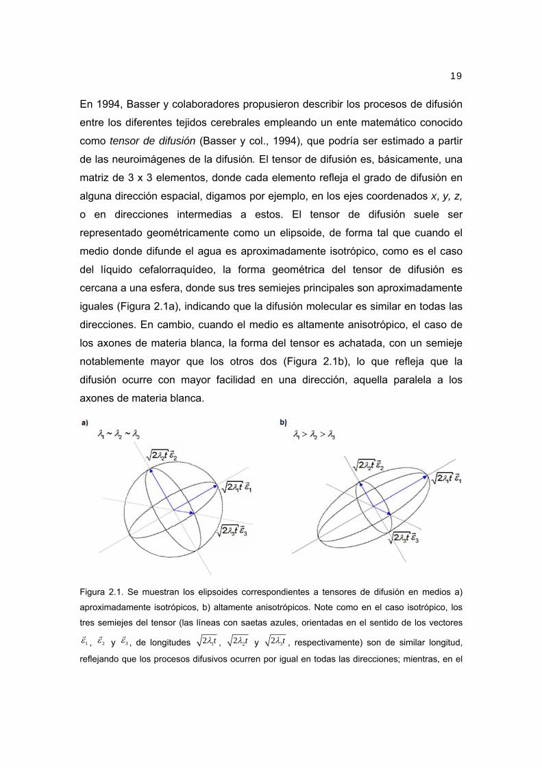
o en direcciones intermedias a estos. El tensor de difusión suele ser
representado geométricamente como un elipsoide, de forma tal que cuando el
medio donde difunde el agua es aproximadamente isotrópico, como es el caso
del líquido cefalorraquídeo, la forma geométrica del tensor de difusión es
cercana a una esfera, donde sus tres semiejes principales son aproximadamente
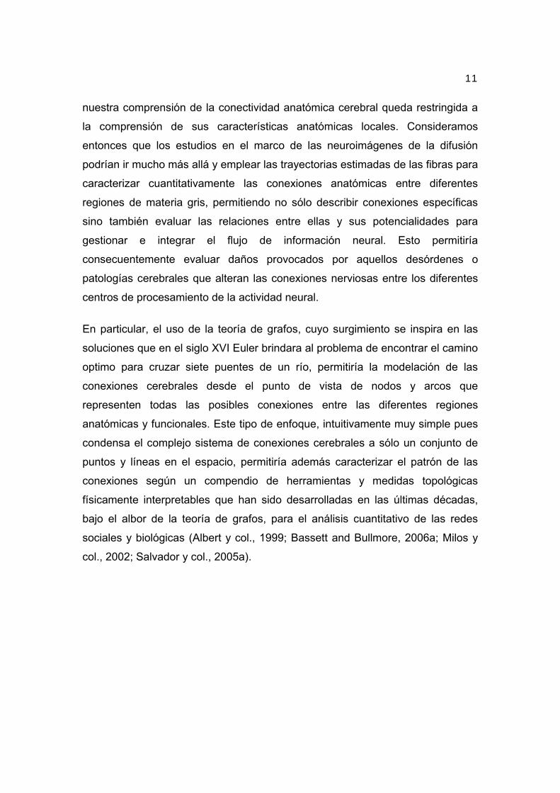
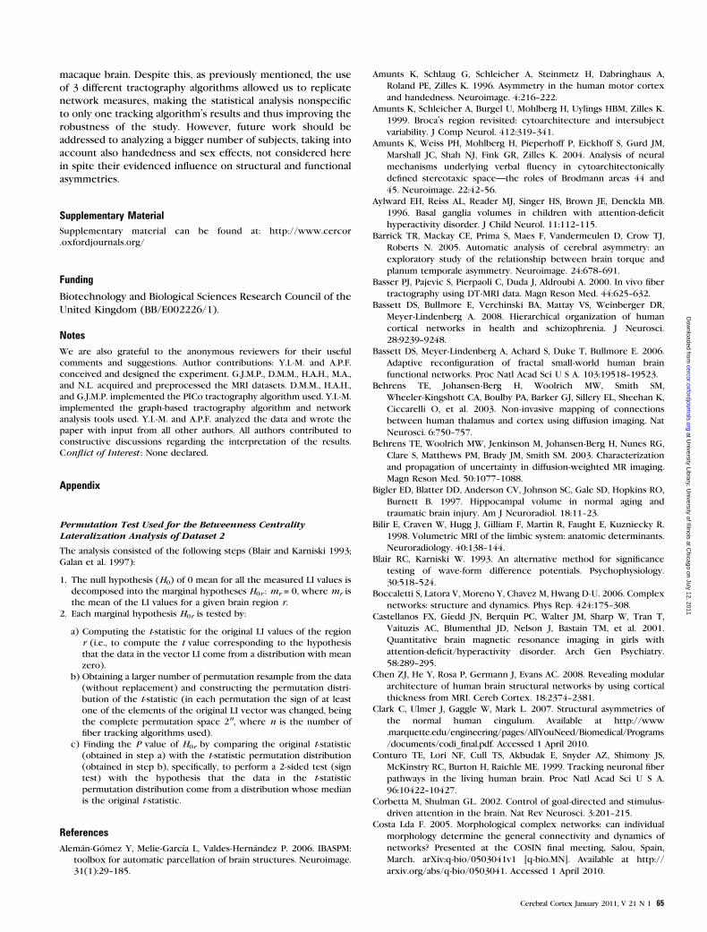
iguales (Figura 2.1a), indicando que la difusión molecular es similar en todas las
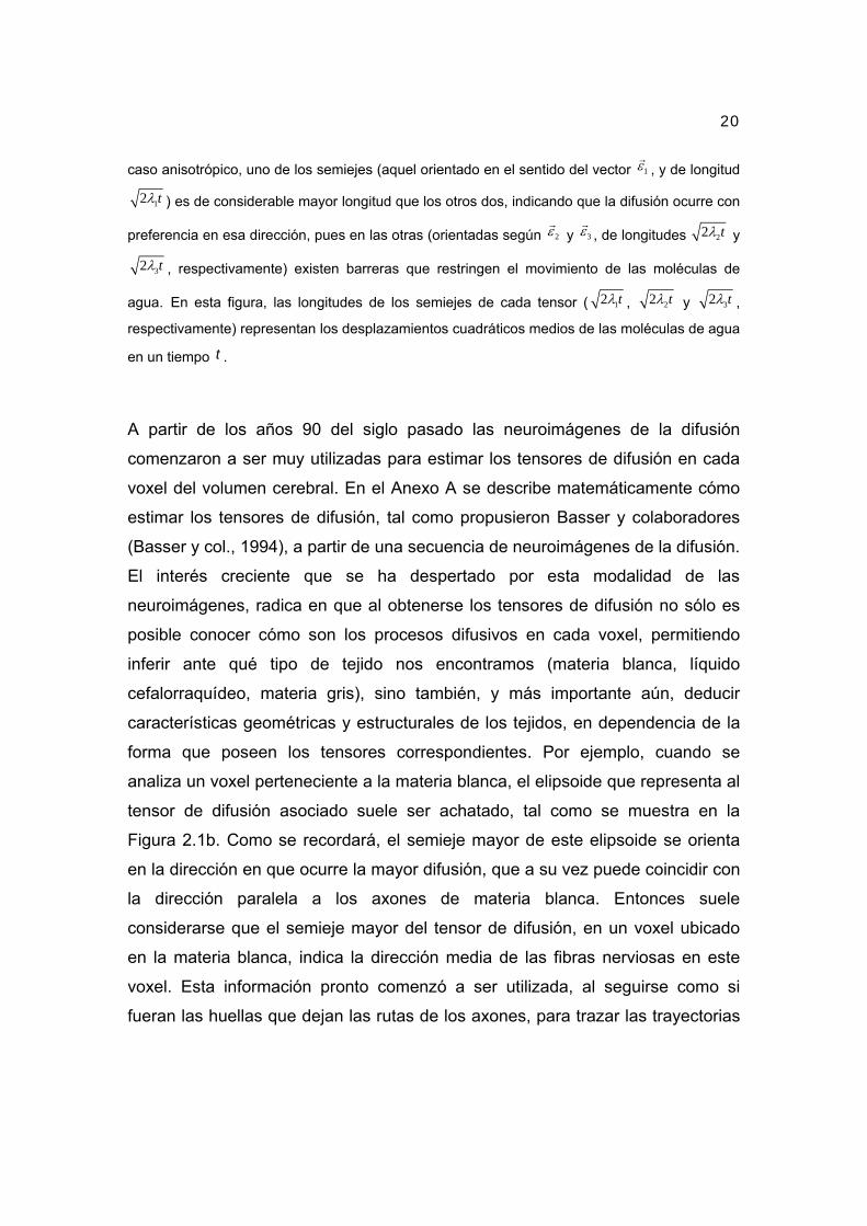
direcciones. En cambio, cuando el medio es altamente anisotrópico, el caso de
los axones de materia blanca, la forma del tensor es achatada, con un semieje
notablemente mayor que los otros dos (Figura 2.1b), lo que refleja que la
difusión ocurre con mayor facilidad en una dirección, aquella paralela a los
axones de materia blanca.
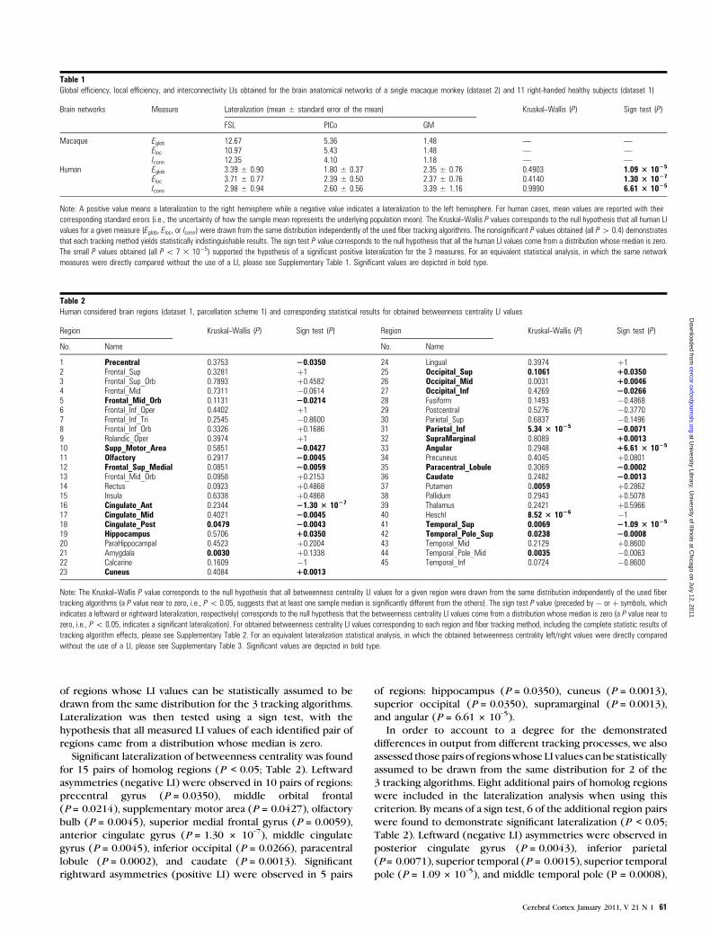
Figura 2.1. Se muestran los elipsoides correspondientes a tensores de difusión en medios a)
aproximadamente isotrópicos, b) altamente anisotrópicos. Note como en el caso isotrópico, los
tres semiejes del tensor (las líneas con saetas azules, orientadas en el sentido de los vectores
1
, 2
y 3
, de longitudes 12 t , 22 t y 32 t , respectivamente) son de similar longitud,
reflejando que los procesos difusivos ocurren por igual en todas las direcciones; mientras, en el
20
caso anisotrópico, uno de los semiejes (aquel orientado en el sentido del vector 1
, y de longitud
12 t ) es de considerable mayor longitud que los otros dos, indicando que la difusión ocurre con
preferencia en esa dirección, pues en las otras (orientadas según 2
y 3
, de longitudes 22 t y
32 t , respectivamente) existen barreras que restringen el movimiento de las moléculas de
agua. En esta figura, las longitudes de los semiejes de cada tensor ( 12 t , 22 t y 32 t ,
respectivamente) representan los desplazamientos cuadráticos medios de las moléculas de agua
en un tiempo t .
A partir de los años 90 del siglo pasado las neuroimágenes de la difusión
comenzaron a ser muy utilizadas para estimar los tensores de difusión en cada
voxel del volumen cerebral. En el Anexo A se describe matemáticamente cómo
estimar los tensores de difusión, tal como propusieron Basser y colaboradores
(Basser y col., 1994), a partir de una secuencia de neuroimágenes de la difusión.
El interés creciente que se ha despertado por esta modalidad de las
neuroimágenes, radica en que al obtenerse los tensores de difusión no sólo es
posible conocer cómo son los procesos difusivos en cada voxel, permitiendo
inferir ante qué tipo de tejido nos encontramos (materia blanca, líquido
cefalorraquídeo, materia gris), sino también, y más importante aún, deducir
características geométricas y estructurales de los tejidos, en dependencia de la
forma que poseen los tensores correspondientes. Por ejemplo, cuando se
analiza un voxel perteneciente a la materia blanca, el elipsoide que representa al
tensor de difusión asociado suele ser achatado, tal como se muestra en la
Figura 2.1b. Como se recordará, el semieje mayor de este elipsoide se orienta
en la dirección en que ocurre la mayor difusión, que a su vez puede coincidir con
la dirección paralela a los axones de materia blanca. Entonces suele
considerarse que el semieje mayor del tensor de difusión, en un voxel ubicado
en la materia blanca, indica la dirección media de las fibras nerviosas en este
voxel. Esta información pronto comenzó a ser utilizada, al seguirse como si
fueran las huellas que dejan las rutas de los axones, para trazar las trayectorias
21
que presentan las fibras nerviosas al conectar las diferentes regiones de materia
gris.
Al procedimiento de reconstruir o poner de manifiesto la trayectoria que
presentan las fibras nerviosas a partir de la información que brindan las
neuroimágenes de la difusión, se le conoce como tractografía, y ha representado
un paso de avance en la descripción in vivo de la anatomía cerebral,
contribuyendo significativamente a la comprensión de los procesos de
integración anatomo-funcional (Koch y col., 2002; LeBihan D. y col., 2001;
Ramnani y col., 2004; Sotero y col., 2007; Sporns y col., 2005). Sin embargo,
desde la propuesta del primer algoritmo de tractografía hasta hoy, han surgido
muchas variantes que tratan de superar las limitaciones propias de cada
algoritmo anterior, así como de aprovechar mejor la información contenida en las
neuroimágenes de la difusión para alcanzar una representación anatómica más
realista. En el Anexo B de esta tesis se describen algunos de los algoritmos más
empleados en el trazado de la trayectoria de las fibras nerviosas. Sin dudas, las
múltiples formas en que estos han sido diseñados reflejan aspectos elementales
a tenerse en cuenta al implementar la tractografía. Pero tal vez el más
significativo de dichos aspectos, y que a su vez marca la diferencia esencial
entre todos los algoritmos, lo constituye la selección adecuada, en cada voxel,
de una dirección de avance que se aproxime lo más posible a la orientación real
de las fibras nerviosas, siendo determinante la función o estrategia que se
utilice. De esto depende la solución que se le dé a configuraciones complejas en
la estructura local de la materia blanca, como pueden ser los cruces, dobleces o
abanicamientos de fibras.
En este sentido, los datos de difusión presentan importantes limitaciones
intrínsecas, dos de las más importantes son: (i) no permiten dilucidar el sentido
de aferencia o eferencia de las fibras, debido a que aunque permiten saber en
qué direcciones difunden las moléculas de agua, no brindan información sobre el
sentido en que ocurre esta difusión para una dirección dada, por lo tanto al
trazar la trayectoria de una fibra no sabemos si lo hacemos a favor o en contra
22
del sentido en que esta fibra conduce los impulsos nerviosos; (ii) existen
múltiples configuraciones para las que puede obtenerse una misma señal de
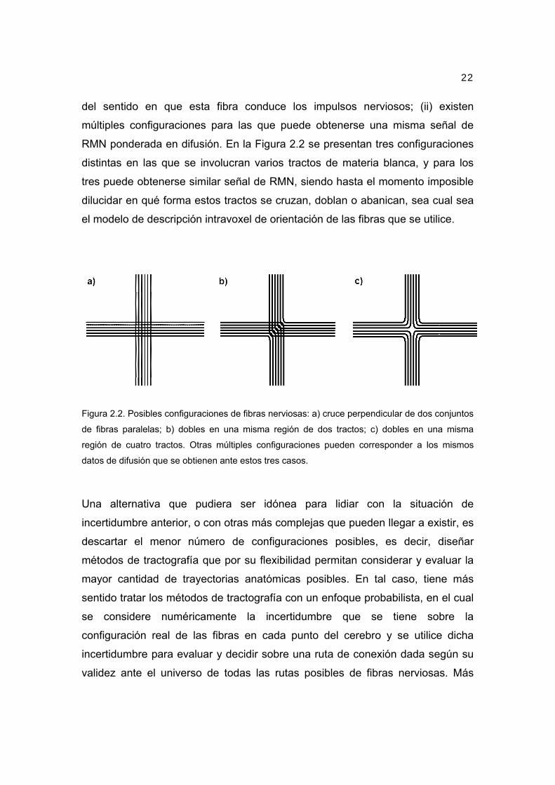
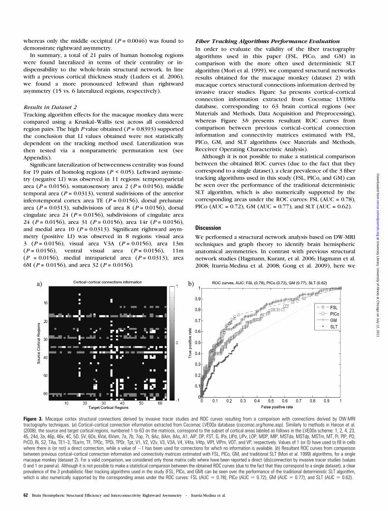
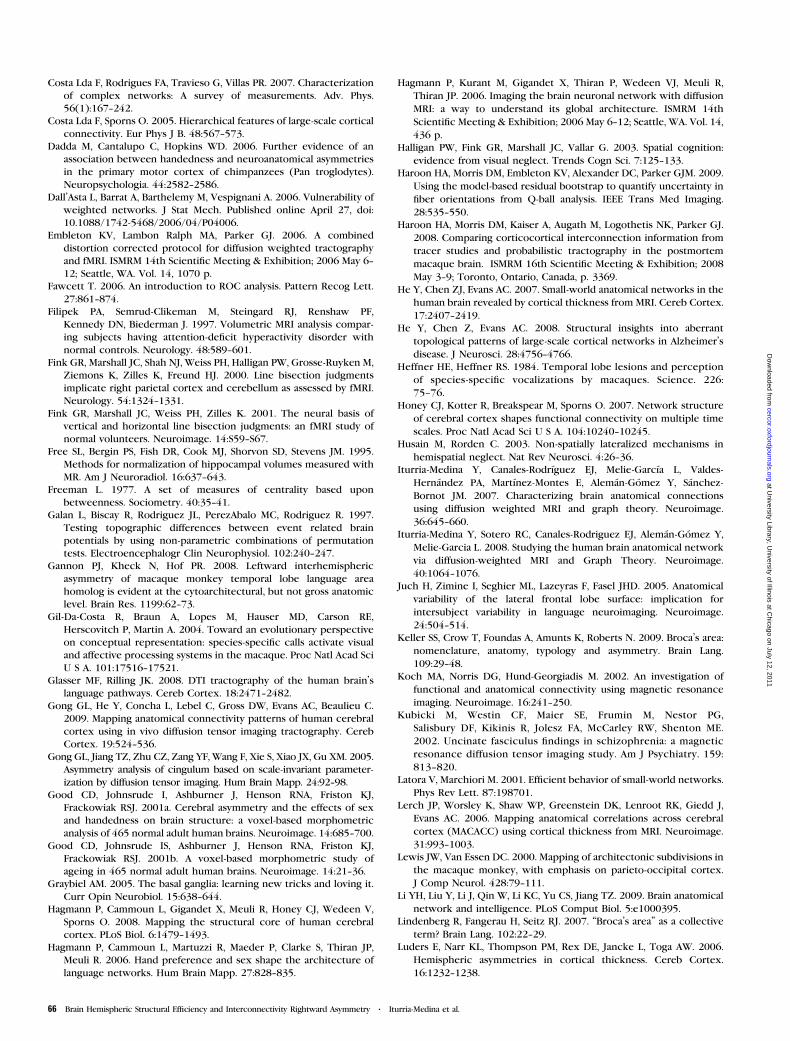
RMN ponderada en difusión. En la Figura 2.2 se presentan tres configuraciones
distintas en las que se involucran varios tractos de materia blanca, y para los
tres puede obtenerse similar señal de RMN, siendo hasta el momento imposible
dilucidar en qué forma estos tractos se cruzan, doblan o abanican, sea cual sea
el modelo de descripción intravoxel de orientación de las fibras que se utilice.
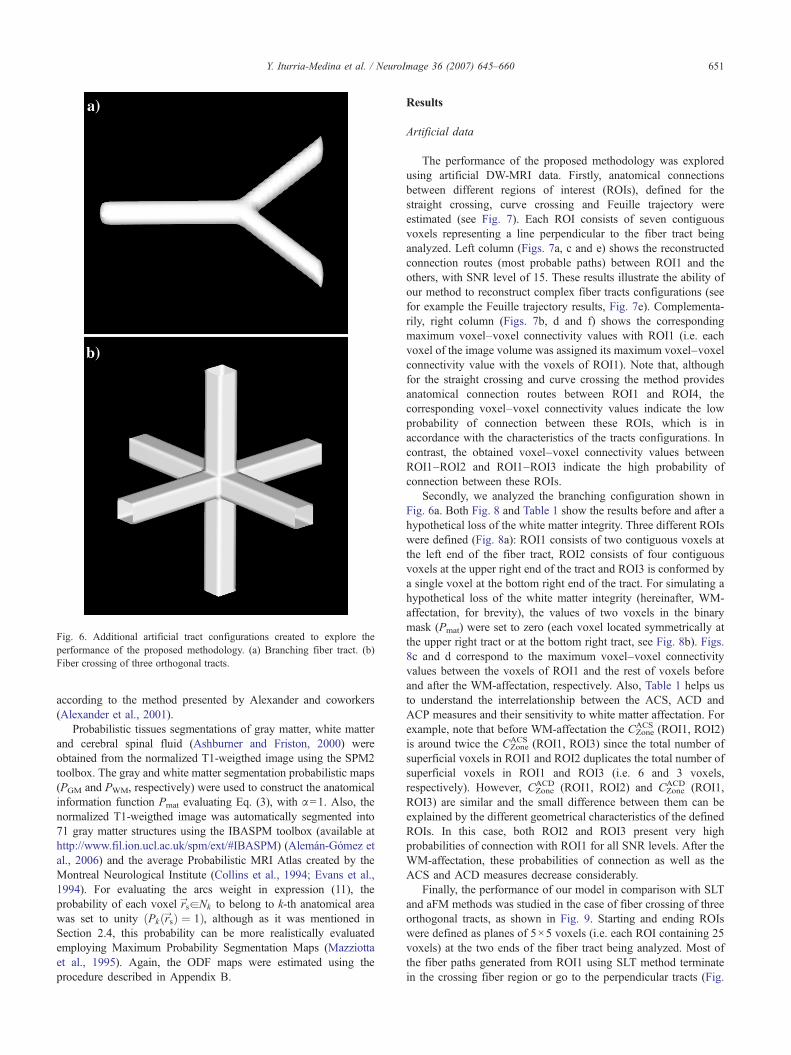
Figura 2.2. Posibles configuraciones de fibras nerviosas: a) cruce perpendicular de dos conjuntos
de fibras paralelas; b) dobles en una misma región de dos tractos; c) dobles en una misma
región de cuatro tractos. Otras múltiples configuraciones pueden corresponder a los mismos
datos de difusión que se obtienen ante estos tres casos.
Una alternativa que pudiera ser idónea para lidiar con la situación de
incertidumbre anterior, o con otras más complejas que pueden llegar a existir, es
descartar el menor número de configuraciones posibles, es decir, diseñar
métodos de tractografía que por su flexibilidad permitan considerar y evaluar la
mayor cantidad de trayectorias anatómicas posibles. En tal caso, tiene más
sentido tratar los métodos de tractografía con un enfoque probabilista, en el cual
se considere numéricamente la incertidumbre que se tiene sobre la
configuración real de las fibras en cada punto del cerebro y se utilice dicha
incertidumbre para evaluar y decidir sobre una ruta de conexión dada según su
validez ante el universo de todas las rutas posibles de fibras nerviosas. Más
23
concretamente, ¿cómo se podría hacer esto?: supongamos que primero
pudiéramos computar un índice que exprese la concordancia de cada camino de
fibra hipotético con la información que ofrecen los datos de difusión, o, en otras
palabras, qué se pudiera cuantificar qué tanta incertidumbre o seguridad hay
sobre las direcciones de las fibras nerviosas a lo largo de un camino de fibra
considerado; luego, si pudiéramos evaluar este índice para todos los caminos de
fibras posibles en el cerebro, entonces podríamos escoger aquel que resulta
más válido, o de menor incertidumbre asociada, metodología que nos permitiría
además considerar esa incertidumbre asociada como una medida de
conectividad anatómica “optimizada” entre dos voxeles cualesquiera del cerebro.
En el Artículo 1, se introduce un método de tractografía diseñado para descartar
el menor número de configuraciones de fibras posibles a la vez que exprese de
forma cuantitativa la conectividad anatómica entre dos puntos cerebrales de
interés. En este, para encontrar la ruta de conexión entre dos voxeles a través
de la materia blanca, se propone analizar el espacio de todas las trayectorias
discretas posibles entre ellos, arribando finalmente al camino que maximice la
conectividad anatómica según el modelo planteado, basándonos en las
facilidades que presenta la teoría de grafos para realizar tal tipo de definiciones.
Otro punto que se tiene en cuenta, según la metodología presentada en el
Artículo 1, y que permite formular directamente la teoría de grafos, es la
caracterización de las conexiones anatómicas entre diferentes estructuras de
materia gris. Aunque en estudios anteriores (Behrens y col., 2003a; Koch y col.,
2002; Parker y col., 2002; Parker y col., 2003; Staempfli y col., 2006; Tuch D.S,
2002), se ha empleado la probabilidad frecuentista de conexión o una métrica de
conectividad anatómica entre sólo dos voxeles, la generalización de esos
conceptos entre regiones anatómicas que poseen cientos de voxeles no es
inmediata. Un trabajo nuestro anterior, que no forma parte de estas tesis (Iturria-
Medina y col., 2005b), propuso cuantificar la fuerza de conexión entre dos
estructuras anatómicas a partir de la información geométrica de los caminos
probabilísticos obtenidos entre estas estructuras. En este se definía la fuerza de
conexión de manera proporcional al área que sobre la superficie de las
24
estructuras ocupan los caminos de fibras nerviosas calculados. Una matriz de
conectividad estimada empleando dicha formulación fue utilizada para acoplar
varias áreas cerebrales en un modelo de masa para la generación del EEG,
obteniéndose resultados fisiológicamente correctos (Sotero y col., 2007).
Específicamente, en el Artículo 1 se emplea la teoría de grafos al introducir, por
primera vez, un modelo grafo de conectividad anatómica cerebral. En un primer
paso, (i) los voxeles del volumen cerebral son considerados nodos de un grafo
pesado no-direccional, en el cual el peso de cada arco que conecta dos nodos
contiguos se asigna según la probabilidad de que ambos nodos se encuentren
conectados por fibras nerviosas. Dicha probabilidad se estima considerando
tanto las segmentaciones probabilistas de tejidos de una imagen anatómica de
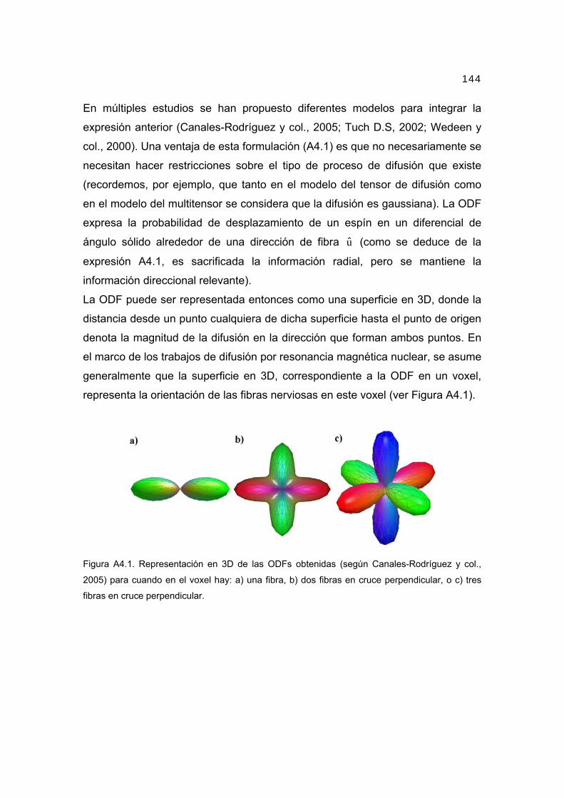
resonancia magnética (por ejemplo, de una imagen ponderada en T1) como una
función, denominada función orientacional de las fibras nerviosas (ODF, del
inglés Orientational Distribuction Function), que expresa en cada voxel la
probabilidad de encontrar un fibra nerviosa en cualquier dirección del espacio y
que es estimada a partir de las señales de RMN ponderadas en difusión. Se
propone entonces un nuevo algoritmo de tractografía, el cual resuelve el
problema del camino más probable entre dos puntos de interés sobre el grafo
definido, y además permite obtener mapas probabilísticos de conectividad
anatómica entre los diferentes voxeles del volumen cerebral. En un segundo
paso, con el objetivo de estimar las conexiones anatómicas entre K estructuras
de materia gris, (ii) el grafo cerebral inicial es tratado como un grafo K+1 partito,
para ello se particiona el conjunto de nodos inicial en K subconjuntos no
solapados de materia gris y un subconjunto que reúne a los nodos restantes
(aquellos que pertenecen a la materia blanca o al líquido cefalorraquídeo).
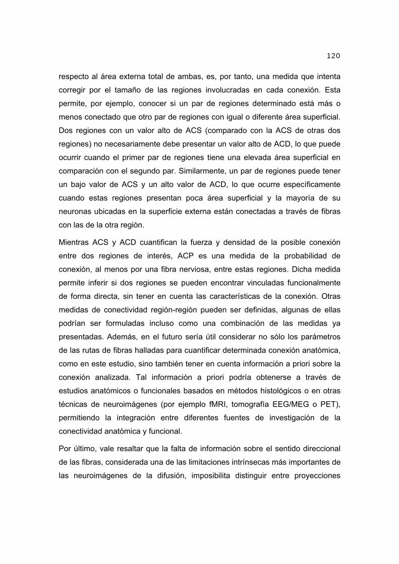
Basado en dicho grafo multipartito, se definen tres medidas de conectividad
entre estructuras: Fuerza de Conexión Anatómica (ACS), Densidad de Conexión
Anatómica (ACD) y Probabilidad de Conexión Anatómica (ACP). ACS es una
medida del flujo potencial de información entre cualquier par de regiones,
considerando que dicho flujo es proporcional a la cantidad de fibras nerviosas
conectoras. DCA es una medida de la fracción del área externa de las regiones
25
que se encuentra conectada con respecto al área externa total de ambas, es,
por ende, una medida que intenta corregir ACS según el tamaño de las regiones
involucradas en la conexión. Por último, ACP es una medida de la probabilidad
de conexión, al menos por una fibra nerviosa, entre cada par de regiones. Esta
refleja, por tanto, si dos regiones de interés se pueden encontrar vinculadas
funcionalmente de forma directa, sin tener en cuenta las características
geométricas (fuerza, densidad) de la conexión.
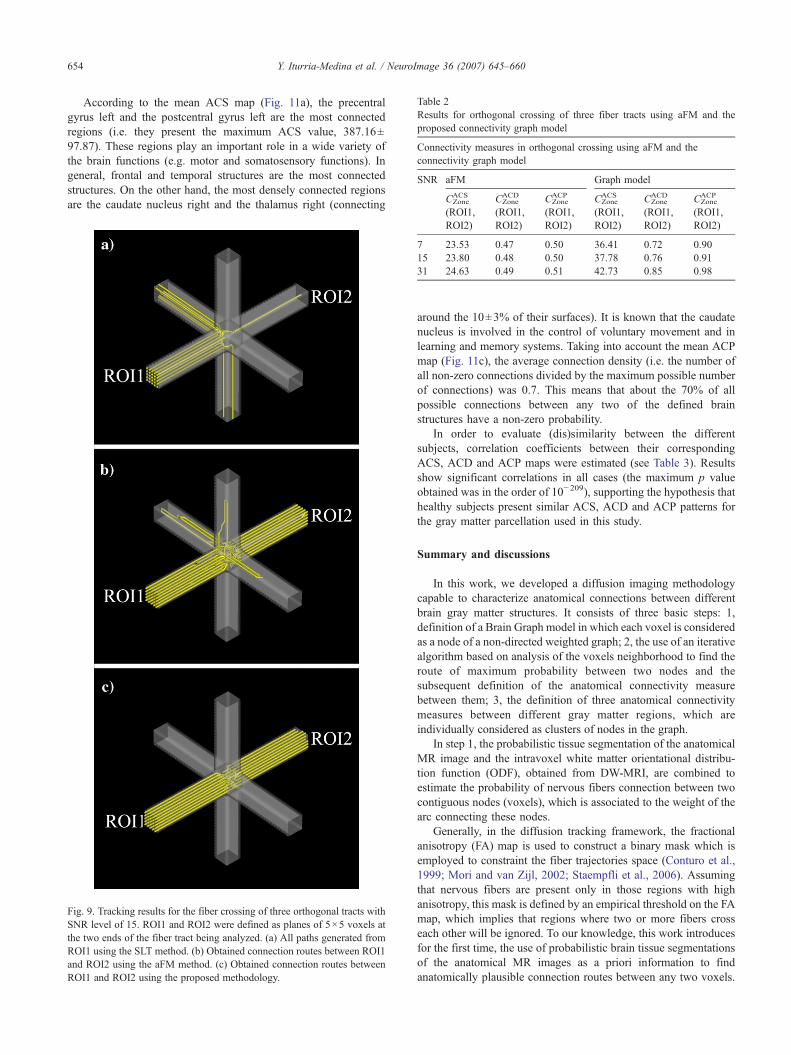
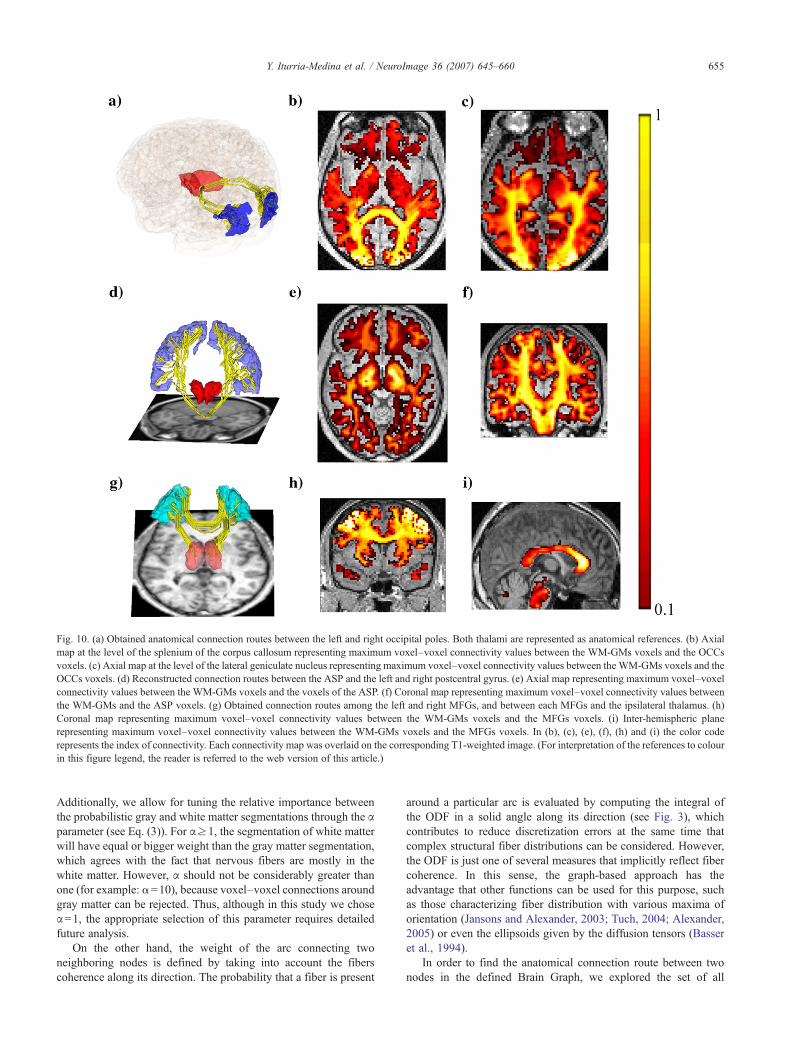
La metodología propuesta es evaluada en datos artificiales y reales. En ambos
casos, los resultados muestran que las trayectorias de las fibras fueron
correctamente reconstruidas entre las regiones de interés. Además, son
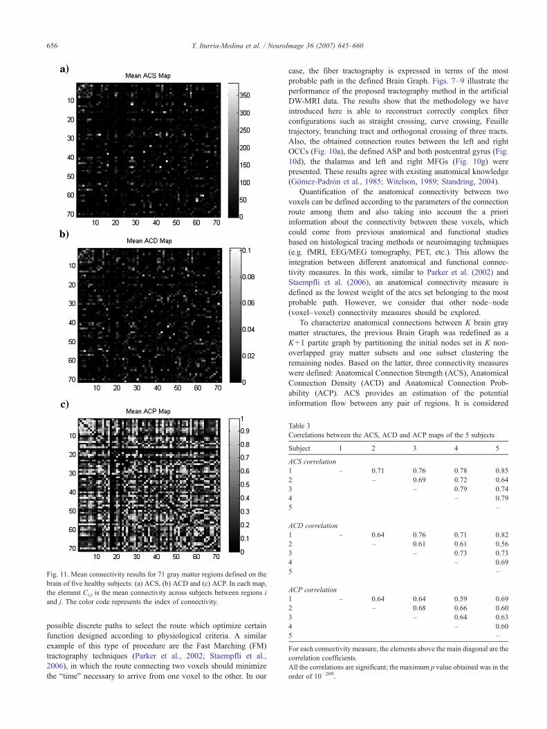
presentados los mapas medios de ACS, ACD y ACP entre 71 estructuras de la
materia gris, para 5 sujetos saludables. Un análisis de correlaciones entre los
mapas individuales de conectividad muestra similaridades significativas entre los
diferentes sujetos, lo que apoya la hipótesis de que individuos sanos deben
presentar patrones similares de conectividad.
26
2.2. CARACTERIZACIÓN TOPOLÓGICA DE LA RED
ANATÓMICA CEREBRAL DE HUMANOS SANOS
Casi de forma paralela al interés creciente en las técnicas basadas en
neuroimágenes de la difusión, ocurrió en la comunidad científica el nacimiento
de una nueva rama de las neurociencias que no tardó en esparcirse: el análisis
topológico de las redes complejas cerebrales. En este tipo de análisis, el cerebro
es modelado como una red compleja compuesta por nodos (puntos en el
espacio) que representan regiones anatómicas o funcionales, y arcos (líneas
que unen a los nodos) que representan las correspondientes conexiones
anatómicas o funcionales. Luego se evalúan un conjunto de medidas topológicas
que pueden ser interpretadas en términos de la disposición cerebral intrínseca,
local o global, para el manejo e integración de la información neural.
Los primeros estudios en el campo de las redes complejas cerebrales (Hilgetag
and Kaiser, 2004; Sporns and Zwi, 2004), se enfocaron básicamente en describir
los atributos de mundo-pequeño (o small-world, en inglés) que presenta la red
de las conexiones anatómicas en algunas especies de mamíferos como gatos y
monos. El concepto de mundo-pequeño, surgió del análisis de las redes sociales
y se asocia a una alta capacidad para intercambiar y procesar información a la
vez que se mantiene un bajo costo de conexiones necesarias (Albert y col.,
1999; Watts, 1999; Watts and Strogatz, 1998). Traducido al ámbito de la
estructura cerebral a nivel macroscópico, aquel correspondiente al de las
conexiones entre áreas anatómica o funcionalmente segregadas, estaría
revelando una alta capacidad para el procesamiento local y global de la
información a expensas de un costo anatómico relativamente bajo (Bassett and
Bullmore, 2006b).
Para realizar los estudios anteriores, donde se revelaría la alta optimización
estructural de las redes definidas por las conexiones anatómicas cerebrales de
27
determinados mamíferos (Hilgetag and Kaiser, 2004; Sporns and Zwi, 2004), se
había empleado sólo información de conectividad anatómica adquirida post
mortem a través de técnicas invasivas (básicamente trazadores radiactivos).
Dichas técnicas invasivas no han sido aplicadas a igual escala en humanos,
debido principalmente a las implicaciones éticas de tales procedimientos, y a las
limitaciones intrínsecas de las metodologías basadas en trazadores radiactivos
para estudiar un cerebro de mayor tamaño y complejidad que el de las otras
especies mencionadas. Luego, la insuficiente información de conectividad
anatómica cerebral reportada para humanos no permitía la caracterización de la
red compleja definida por sus conexiones cerebrales. Sin embargo, ya en el año
2006 se emplearon técnicas basadas en neuroimágenes de la difusión para
crear el primer mapa de conexiones anatómicas posibles entre pequeñas
regiones que cubrían toda la materia gris de un humano sano (Hagmann y col.,
2006). Para ello se trazaron las trayectorias de fibras que unían a las regiones
de materia gris, y se consideró que cada región era representada por un nodo y
que dos nodos cualesquiera (o regiones) estaban unidos por un arco si existía
entre ellos una conexión de materia blanca, según las trayectorias de fibras
reconstruidas. Los resultados de dicho estudio, basados principalmente en el
análisis de algunas propiedades básicas de la red compleja obtenida, apoyaron
el punto de vista de que el cerebro humano, a semejanza del de otras especies
de mamíferos, está optimizado estructuralmente para lograr un elevado
procesamiento local y global de la información, con un bajo costo de conexiones
necesarias, cumpliendo con el principio de mundo-pequeño. Pero, a pesar de su
originalidad y relevancia científica, este estudio presentó algunas limitaciones
metodológicas notables, como el empleo de un solo sujeto, el análisis de sólo
algunas pocas propiedades topológicas de la red, y la aproximación de esta red
a un formato binario en el que se desprecia el peso o la evidencia numérica
sobre la existencia de las conexiones estimadas (asumiendo que todas tienen
igual valor).
28
A continuación, He y colaboradores (2007) propusieron estudiar patrones de
conectividad reflejados en los cambios concurrentes en el grosor cortical de
diferentes estructuras corticales (He y col., 2007). Dicho estudio se basó en la
hipótesis de que dos regiones conectadas anatómicamente presentan
características similares en cuanto al tipo de tejido que poseen, pues deben
procesar información similar, y por ello debe esperarse que algunas de sus
características geométricas se modifiquen de forma concurrente (por ejemplo el
grosor cortical, que se asocia al ancho de las capas que componen las columnas
corticales y subsecuentemente a la cantidad de neuronas contenidas en estas).
Las cortezas cerebrales de 124 sujetos saludables fueron divididas en 54
estructuras típicas, definidas antes de acuerdo a criterios anatómicos y
funcionales, y entonces dos estructuras cualesquiera fueron consideradas
conectadas si existía una correlación significativa en la manera en que variaban
sus grosores corticales a lo largo de todos los sujetos. Los resultados que se
obtuvieron apoyaron también la hipótesis de que el cerebro humano está
organizado estructuralmente siguiendo los principios de mundo-pequeño, así
como también siguiendo otros atributos que implican una alta optimización, pero
no podrían ser resultados concluyentes al respecto porque, entre otras causas,
la metodología empleada no permitió incluir estructuras subcorticales internas,
como los tálamos o las amígdalas, las cuales mantienen conexiones
elementales con la corteza cerebral. No fue posible además obtener la red
correspondiente a cada sujeto sino sólo una red global representando a toda la
muestra, que a su vez, como en el estudio de Hagmann y colaboradores, fue
analizada también sin considerar el peso o la evidencia numérica sobre la
existencia de las conexiones estimadas.
En el Artículo 2, se continúa la caracterización de la red compleja constituida por
las conexiones anatómicas en el cerebro humano. Para ello se extienden los
trabajos pioneros de Hagmann y He anteriormente mencionados en varios
puntos: 1) en lugar de crear una red binaria, se construye y analiza una versión
pesada, donde el peso de cada conexión es asignado según la Probabilidad de
29
Conexión Anatómica (ACP) entre los pares de regiones consideradas, medida
definida con anterioridad en el Artículo 1, que expresa la probabilidad de que dos
regiones cualesquiera estén conectadas por al menos una fibra nerviosa; 2) se
mapean las conexiones entre 90 estructuras corticales y subcorticales,
cubriendo toda la materia gris de 20 humanos saludables, seleccionadas de
acuerdo a criterios anatómicos y funcionales (Tzourio-Mazoyer y col., 2002); 3)
además de evaluar atributos de mundo-pequeño y grado de la distribución,
reportadas en los dos estudios anteriores, otras medidas topológicas de las
redes son evaluadas, como eficiencia, vulnerabilidad, centralidad nodal y
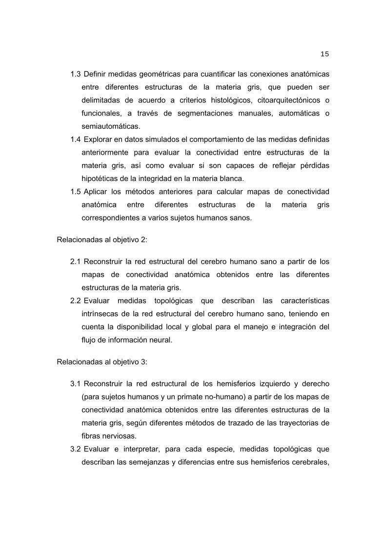
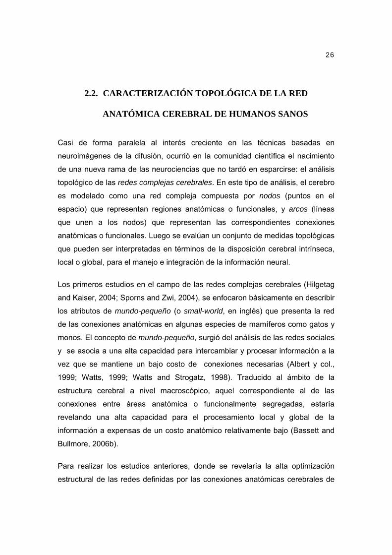
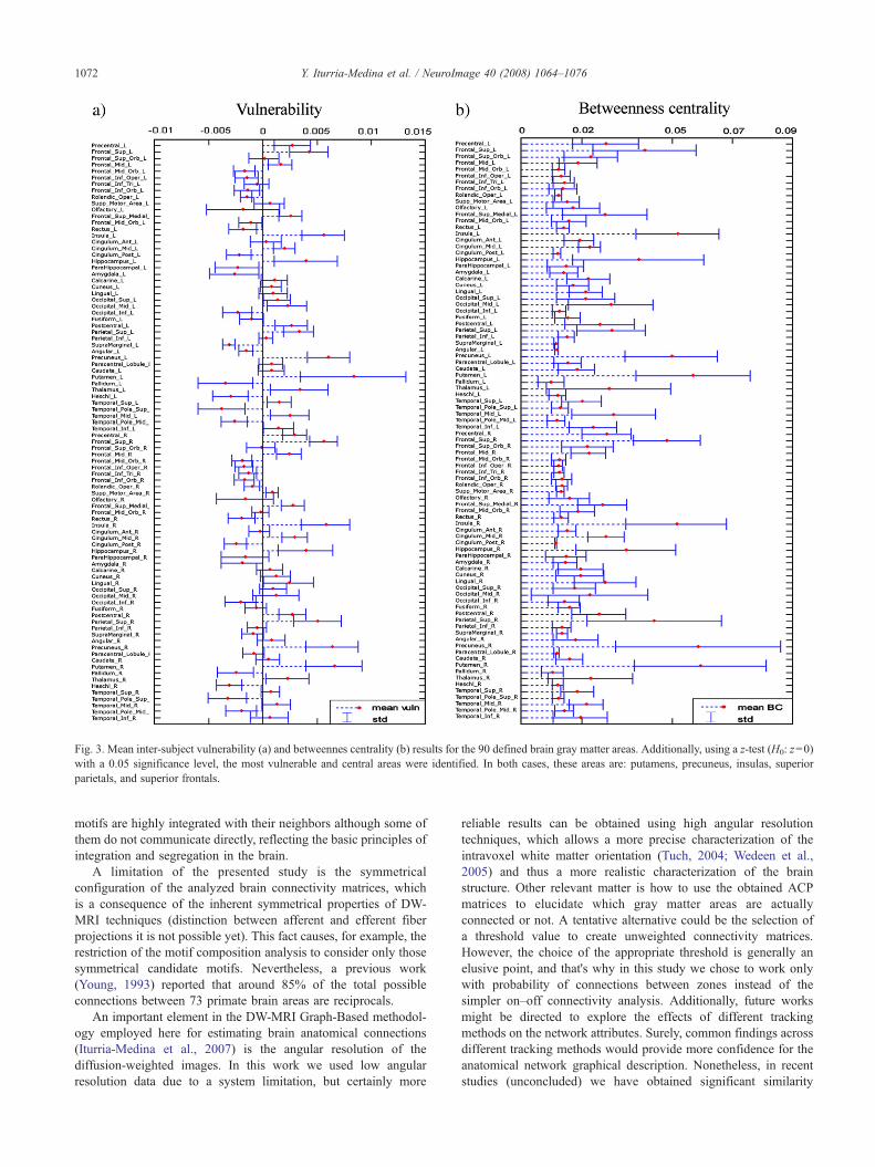
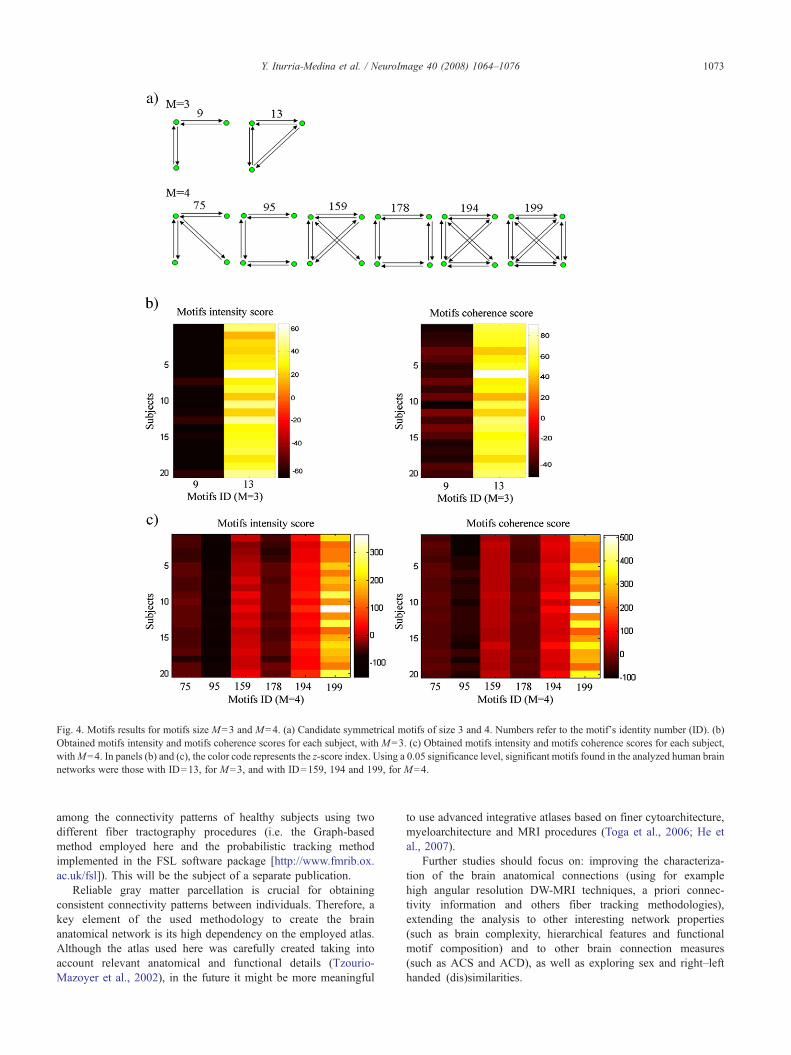
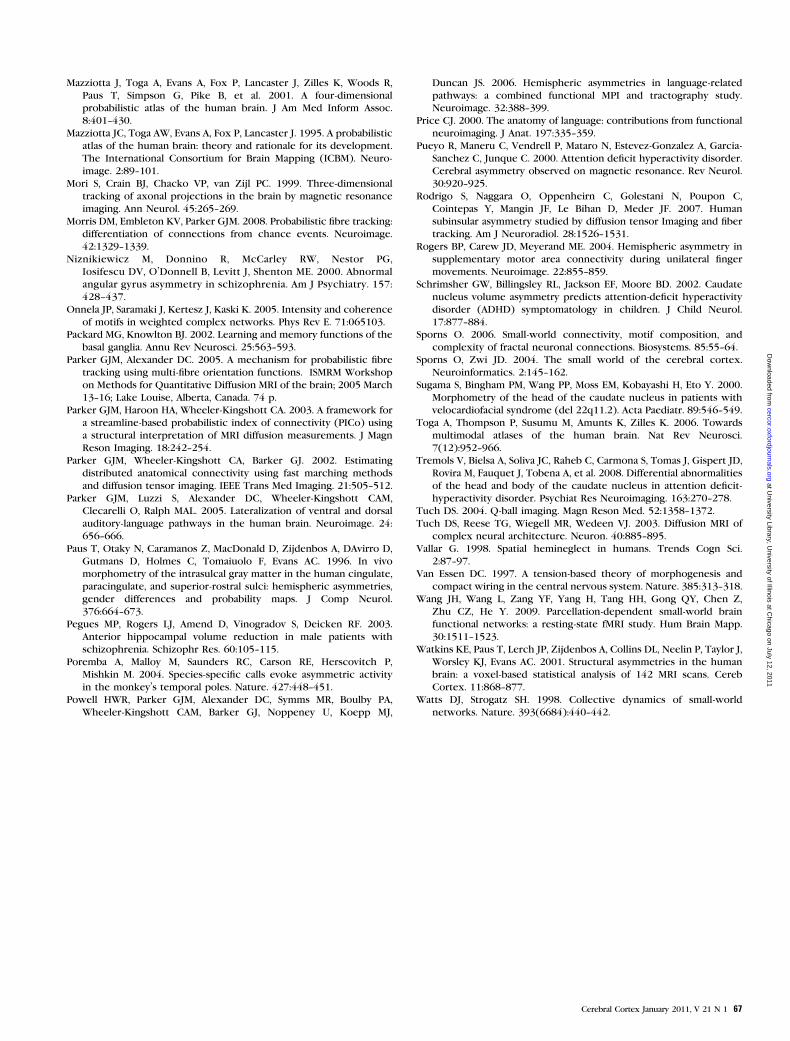
composición de motivos estructurales. En la Figura 2.3 se ilustra de forma
general el procedimiento empleado para la reconstrucción de las redes
anatómicas.
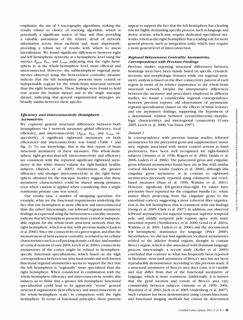
Figura 2.3. Reconstrucción de la red anatómica cerebral. a) Primeramente se estiman las
trayectorias de las fibras nerviosas que conectan las diferentes regiones anatómicas (de acuerdo
al algoritmo presentado en el Artículo 1), en este caso se muestran las trayectorias obtenidas
entre los tálamos y los giros frontales superiores. b) Se crea una matriz donde el elemento
correspondiente a la fila i y a la columna j expresa la probabilidad de que exista conexión entre
las regiones i y j (según la medida PCA definida también en el Artículo 1), en este caso se
muestra una matriz de conectividad entre 90 estructuras anatómicas. c) Finalmente la red
pesada se crea definiendo un punto (nodo) en el espacio por cada región anatómica considerada
y enlazando este a través de líneas (arcos) a aquellas regiones con las que se encuentra
conectado por trayectorias de fibras nerviosas, siendo el grosor de cada línea proporcional al
peso (probabilidad o densidad) de la conexión que representa.
30
Los resultados mostraron que la red anatómica obtenida para cada sujeto
presenta los atributos de mundo-pequeño, con poca variabilidad entre los
sujetos. Esto apoya el punto de vista de que el atributo de mundo-pequeño es
una propiedad común de las redes anatómicas cerebrales correspondientes a
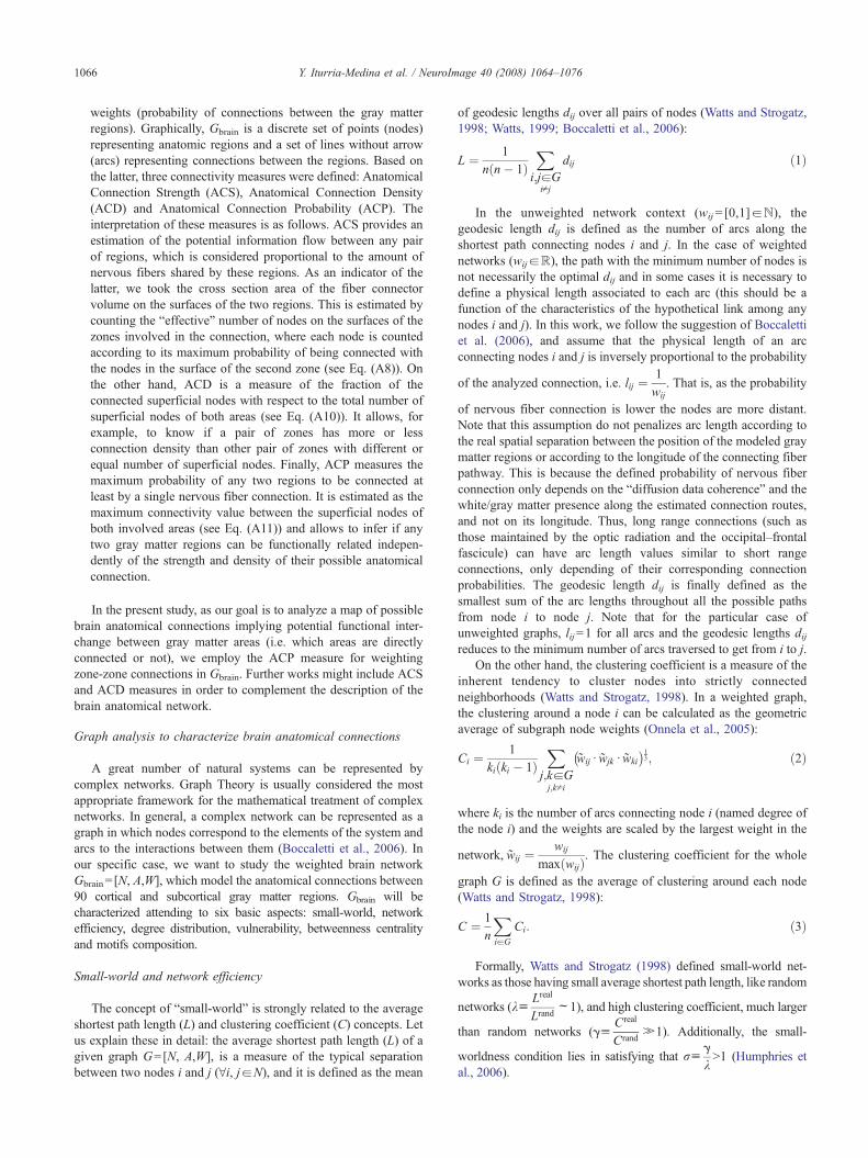
los seres humanos sanos. También se comprobó, a través de la medida grado
de la distribución, que la posibilidad de que una región específica esté conectada
con un número creciente de otras regiones disminuye a medida que aumenta el
número de regiones, comportamiento conocido como de escala-amplia (o broad-
scale, en inglés). El comportamiento de escala-amplia encontrado sugiere un
límite relativamente bajo en la cantidad de conexiones anatómicas que puede
mantener cualquier región cerebral. Este resultado presenta cierta analogía con
la conducta descrita para las redes de amigos, en las que si una persona tratara
de incrementar constantemente su número de amigos tendería también a
descuidar la calidad de las relaciones con ellos, por lo que de forma intuitiva
prefiere mantener un número limitado de amistades iniciales o de restablecer
prioridades entre estas y quienes va conociendo.
El análisis de eficiencia reveló que las redes obtenidas presentan menor
eficiencia global y mayor eficiencia local que sus redes aleatorias equivalentes
(aquellas que presentan igual cantidad de conexiones pero distribuidas
aleatoriamente). Este hallazgo coincidió con lo observado, en el mismo estudio,
para las redes cerebrales de gatos y macacos, así como con lo reportado
previamente para redes funcionales en humanos creadas a partir de imágenes
funcionales de RMN (Achard and Bullmore, 2007). Aunque no existe un
consenso sobre su significado, pudiera estar indicando que el cerebro ha
evolucionado tratando de mantener una eficiencia local alta, lo que es
equivalente a priorizar el intercambio entre regiones que procesan similar
información neural, mientras que a la vez optimiza el costo de los procesos de
integración al garantizar sólo una eficiencia global intermedia, pues no es
necesario el intercambio de información entre todas las regiones cerebrales.
31
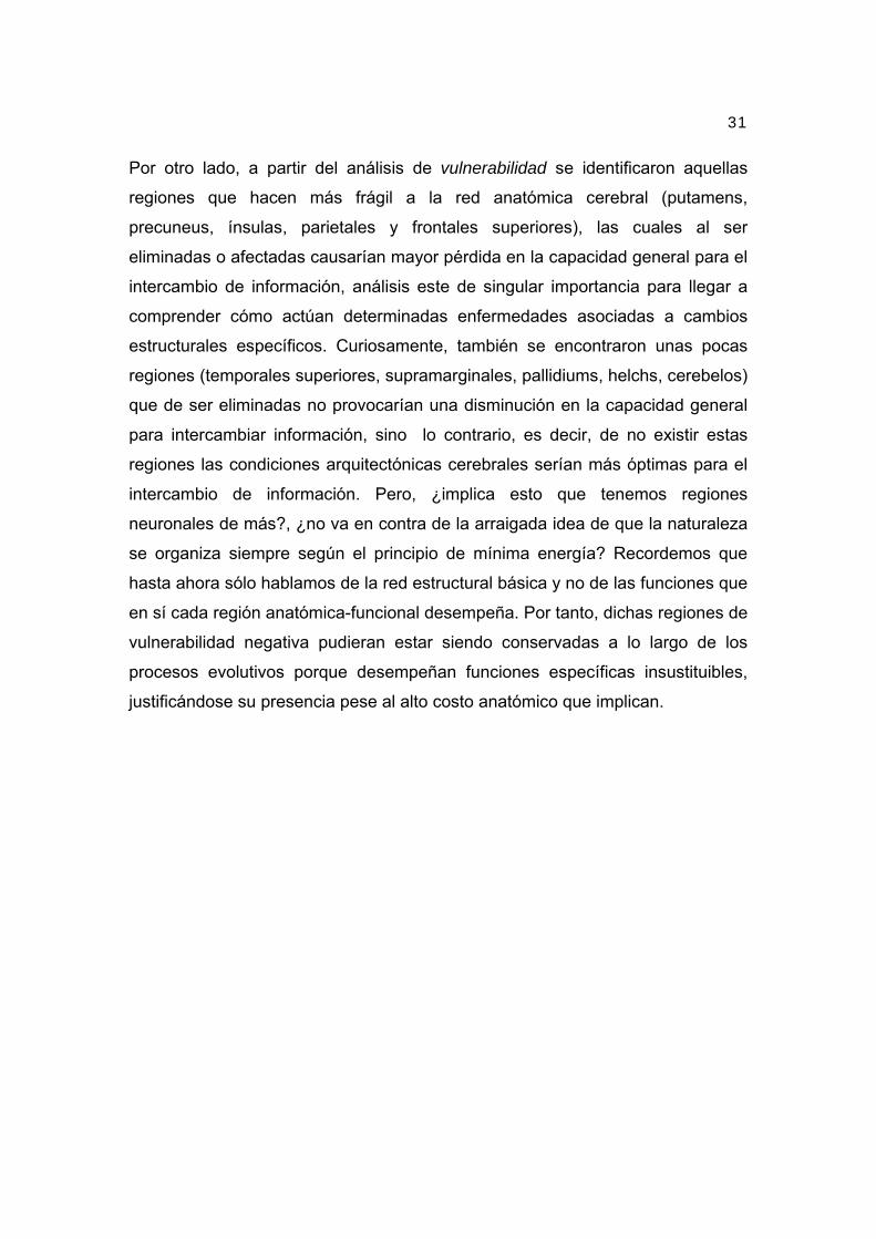
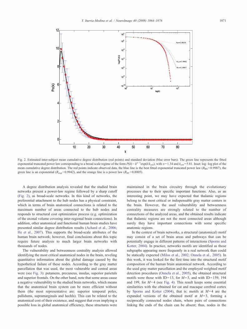
Por otro lado, a partir del análisis de vulnerabilidad se identificaron aquellas
regiones que hacen más frágil a la red anatómica cerebral (putamens,
precuneus, ínsulas, parietales y frontales superiores), las cuales al ser
eliminadas o afectadas causarían mayor pérdida en la capacidad general para el
intercambio de información, análisis este de singular importancia para llegar a
comprender cómo actúan determinadas enfermedades asociadas a cambios
estructurales específicos. Curiosamente, también se encontraron unas pocas
regiones (temporales superiores, supramarginales, pallidiums, helchs, cerebelos)
que de ser eliminadas no provocarían una disminución en la capacidad general
para intercambiar información, sino lo contrario, es decir, de no existir estas
regiones las condiciones arquitectónicas cerebrales serían más óptimas para el
intercambio de información. Pero, ¿implica esto que tenemos regiones
neuronales de más?, ¿no va en contra de la arraigada idea de que la naturaleza
se organiza siempre según el principio de mínima energía? Recordemos que
hasta ahora sólo hablamos de la red estructural básica y no de las funciones que
en sí cada región anatómica-funcional desempeña. Por tanto, dichas regiones de
vulnerabilidad negativa pudieran estar siendo conservadas a lo largo de los
procesos evolutivos porque desempeñan funciones específicas insustituibles,
justificándose su presencia pese al alto costo anatómico que implican.
32
2.3. COMPARACIÓN, EN HUMANOS Y UN PRIMATE NO-
HUMANO, DE LAS REDES ANATÓMICAS DEL HEMISFERIO
DERECHO E IZQUIERDO EN CUANTO A EFICIENCIA Y
OPTIMIZACIÓN ESTRUCTURAL PARA LIDEAR CON EL
FLUJO DE INFORMACIÓN NEURAL
La simetría es considerada una de las componentes indispensables de
perfección y belleza. Sin embargo, tal vez para reafirmarnos lo vano de aspirar a
lo perfecto, ninguna de las formas presentes en la naturaleza es en realidad
simétrica. Por el contrario, los conceptos de simetría y asimetría,
complementarios entre sí, parecen estar siempre en pugna continua por un
escalón dominante. Incluso nuestro cerebro, cuyo mayor atributo es la
complejidad, y es constituido por dos hemisferios aparentemente iguales, no
pudo escapar a esta lucha y revela cada vez más su carácter asimétrico. En
1861, el investigador francés Paul Broca realizó la primera descripción detallada
de asimetría funcional en el cerebro humano. Este encontró una lesión post-
mortem en el hemisferio izquierdo de un paciente que había presentado serias
dificultades para hablar y consecuentemente Broca infirió que las habilidades
para el lenguaje estaban lateralizadas (Broca, 1861). Alrededor de una década
después Carl Wernicke, de origen polaco, reportó que el daño a una zona
específica del hemisferio izquierdo podría causar también una seria afectación
en la comprensión del lenguaje (Wernicke, 1874). Estos fueron los hechos
iniciales que comenzarían la fascinante e inconclusa historia por revelar los
misterios de la asimetría cerebral.
En el capítulo anterior de esta tesis hemos validado la propuesta realizada en el
capítulo 1 de caracterizar la red de conexiones anatómicas cerebrales mediante
la combinación de neuroimágenes de la difusión con elementos de la teoría de
grafos. El próximo paso investigativo que nos ocupa y se presenta en el Artículo
33
3, tal y como sucede en la ciencia que discurre desde la ciencia básica hacia la
aplicada, va entonces en el sentido de su utilización práctica. En un primer
intento de abordaje de un problema práctico, se aplica la metodología descrita al
tema de las asimetrías cerebrales comentado anteriormente. Resulta atractivo
este tópico ya que con antelación, desde Broca y Wernicke hasta nuestros días,
sólo se han explorado las asimetrías estructurales entre aquellas regiones que
soportan funciones conocidas como muy lateralizadas (por ejemplo el lenguaje).
Es decir, la investigación precedente se ha limitado a parear las conocidas
lateralizaciones funcionales con su correspondiente asimetría en las conexiones
de sustancia blanca entre las regiones que soportan esa función. Sin embargo,
nosotros tenemos la posibilidad de caracterizar las asimetrías considerando no
sólo regiones específicas, sino incluyendo a todo el hemisferio cerebral y su
compleja red de conexiones. Además, la caracterización en términos de la teoría
de grafo nos brindaría información no sólo en términos anatómicos, sino también
en el sentido más general y fisiológico del manejo e integración del flujo de
información neural.
Para lograr ese objetivo, se construyeron las redes cerebrales de cada
hemisferio cerebral por separado. Se desprecian por lo tanto aquellas regiones
comunes como el cuerpo calloso, el cual no está lateralizado ya que en sí su
estructura consiste en el cruce de los axones desde un hemisferio cerebral a
otro. La comparación numérica de las propiedades globales de estas redes
hemisféricas muestran, tanto para un grupo de humanos sanos como para un
primate-no humano, a un hemisferio derecho más interconectado y eficiente que
el izquierdo. Además, en términos de la indispensabilidad de cada región
cerebral en específico para el funcionamiento de la red global, se muestra a
través de un índice de lateralización que el hemisferio izquierdo cuenta con más
regiones consideradas como muy indispensables para el funcionamiento de la
red como un todo. Estos dos resultados están en correspondencia con los
conocidos hechos de que el hemisferio derecho tiene un rol principal en aquellos
procesos más generales como las tareas de integración, mientras que el
34
hemisferio izquierdo tiene un rol principal en aquellos procesos específicos
altamente demandantes como el lenguaje o las tareas motoras, que puedan
requerir redes especializadas dedicadas a ellos. Resumiendo, el empleo de
nuestra metodología basada en neuroimágenes de la difusión y teoría de grafos
ha contribuido a proponer una posible explicación sobre el hecho de cuáles
pueden ser las posibles ventajas evolutivas que confiere un cerebro lateralizado,
algo en lo que hasta ahora no existe consenso. Por último vale destacar que,
entre las salidas prácticas, en este artículo por primera vez se expone una
explicación al por qué de la ocurrencia de fenómenos neuropsicológicos luego
de lesión en determinadas regiones cerebrales en un hemisferio cerebral sí y en
otro no.
35
2.4. DISCRIMINACIÓN AUTOMÁTICA DE UNA CONDICIÓN CEREBRAL
PATOLÓGICA TENIENDO EN CUENTA LAS PROPIEDADES
TOPOLÓGICAS DE LA RED ANATÓMICA CEREBRAL
Para un diagnóstico clínico se requiere por lo general de la intervención de un
experto con cuyo criterio se discierna el casi siempre confuso límite entre lo
normal y lo atípico. Sin embargo, muchas veces la tarea del experto se dificulta
ante determinada patología cuyos efectos pueden ser: i) desconocidos, por la
ausencia de literatura previa relacionada, o ii) poco evidenciables a simple vista,
debido a complejidades asociadas a la observación objetiva de la anomalía
correspondiente. Esta difícil situación ocurre con frecuencia ante muchas
patologías neurológicas, como en el caso de la Esclerosis Múltiple o la
Enfermedad de Alzheimer, donde un comportamiento determinado del sujeto y la
evaluación de variables cognitivas relacionadas inducen a considerar la
presencia o agravamiento de alguna patología específica, pero no es posible
confirmar las sospechas debido a la falta de evidencia estructural sobre
afectaciones concretas a los tejidos que suelen ser modificados por esa
patología. En el caso específico de la enfermedad de Alzheimer, el diagnóstico
definitivo sólo se alcanza mediante una biopsia cerebral, que pocas veces se
realiza, debido al desbalance entre coste-beneficio (es muy invasiva). El
diagnóstico queda por tanto en un punto de incertidumbre intermedio, donde,
pese a la falta de evidencia científica suele arriesgarse un tratamiento clínico, en
ocasiones para no dejar de hacer “algo”, cuya efectividad queda a merced de la
futura mejora o empeoramiento del paciente.
Serían de gran ayuda entonces herramientas que contribuyan a hacer el
diagnóstico por sí solas o al menos a mejorar significativamente al diagnóstico
del especialista. Pero, siendo objetivos, ¿podría una de estas herramientas
decirnos cuantitativamente si un sujeto ha dejado de ser saludable, o si empeora
o progresa ante un determinado tratamiento clínico? El anhelo de contar con
tales herramientas se refleja desde hace años en la comunidad científica a
36
través de la búsqueda de biomarcadores: características que son evaluadas y
medidas como indicadores de procesos biológicos normales, procesos
patológicos o respuestas farmacológicas, con el fin de contribuir a la intervención
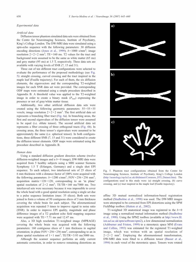
Keywords: Brain connectivity; Diffusion weighted magnetic resonanceimaging; Graph model; Tractography
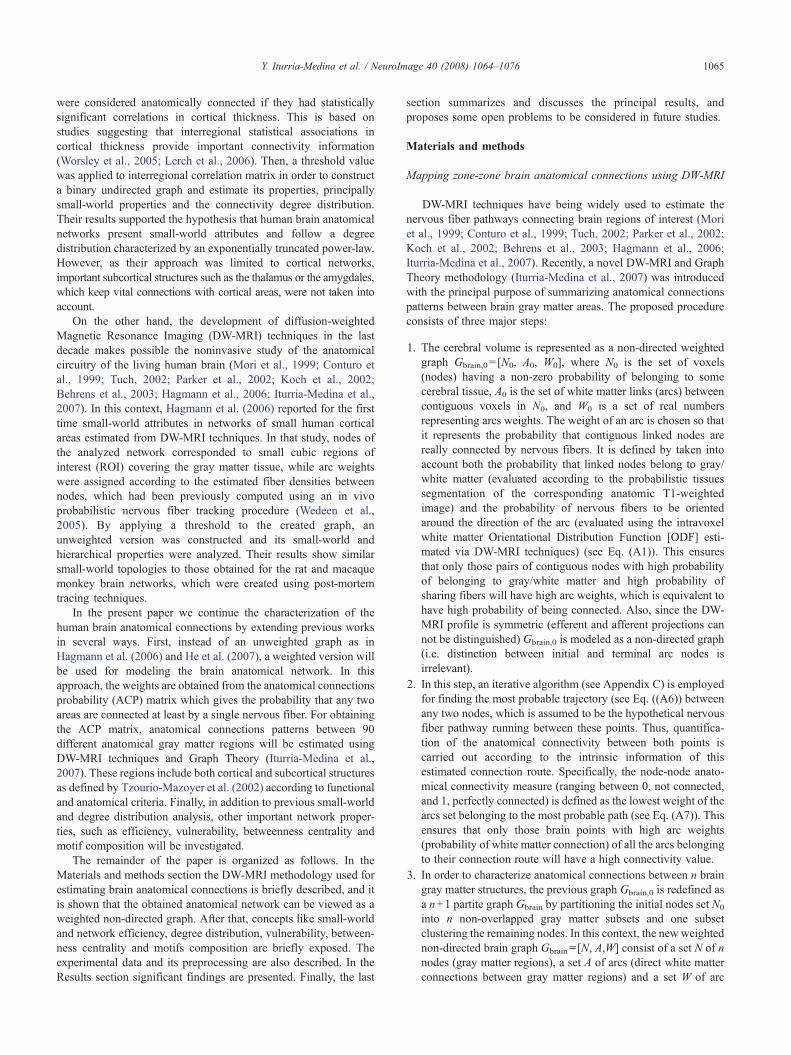
Introduction
Random motion of water molecules inside the brain isinfluenced by the architectural properties of tissues. Waterdiffusion is known to be highly anisotropic in certain white matter
regions, with preferential movement along the nervous fibers. Arecent development of a non-invasive technique which quantifieswater diffusion process, known as Diffusion Weighted MagneticResonance Imaging (DW-MRI), has allowed to obtain structuralinformation about the intravoxel axon arrangement (Basser et al.,1994; LeBihan, 2003). Based on this information, fiber tracto-graphy arises as a crucial technique to attain a better in vivoanatomical characterization of the brain (Mori et al., 1999; Conturoet al., 1999; Tuch, 2002; Parker et al., 2002; Koch et al., 2002;Behrens et al., 2003). Also, quantification of the anatomicalconnectivity between different gray matter structures would be asignificant contribution to the understanding of functional integra-tion of the human brain (LeBihan et al., 2001; Koch et al., 2002;Ramnani et al., 2004; Sporns et al., 2005; Sotero et al., 2007).
Reconstruction of nervous fiber trajectories is an extensivelytreated topic. In the traditional Streamline Tractography (SLT)approach (Mori et al., 1999; Conturo et al., 1999; Basser et al.,2000), a continuous trajectory is traced tangential to the direction ofthe principal eigenvector of the diffusion tensor measured at eachvoxel using a discretization step smaller than the size of the voxel.This approach usually fails in voxels where fibers cross each other,merge, kiss or diverge, and it is very sensitive to the influence ofMR signal noise (Basser and Pajevic, 2000; Lori et al., 2002). Inthose situations, traced path strays from the real trajectory ofnervous fibers. To overcome these limitations, modified StreamlineTractography (mSLT) methods based on Diffusion Tensor Deflec-tion (Weinstein et al., 1999; Lazar et al., 2003) and ProbabilisticMonte-Carlo Method (Parker and Alexander, 2003) have beenproposed. The former uses the entire diffusion tensor to deflect thepropagation direction computed in the previous step. The latter usesthe uncertainty of the estimated nervous fiber orientation to computea large number of possible paths from the seed point; a quantity canbe assigned to each path reflecting some connectivity relationshipbetween seed and target points.
In recent years, many other mSLT methods have been proposed(Tuch, 2002; Tench et al., 2002; Behrens et al., 2003; Hagmannet al., 2003). Usually, they define the anatomical connection pro-
646 Y. Iturria-Medina et al. / NeuroImage 36 (2007) 645–660
bability between seed and target voxels as the ratio between thenumber of shared paths and the number of generated paths.
In contrast to SLT and mSLT methods, Level Set-Based FastMarching (FM) techniques (Parker et al., 2002; Staempfli et al.,2006) express the tractography in terms of a wave front thatemanates from a source point and whose evolution is controlled bythe diffusion data. FM methods have two advantages over the SLTand mSLT methods: 1, better performance in situations ofbranching and fiber crossing, and 2, direct estimation of theprobability of white matter connectivity between two points (JunZhang et al., 2005).
In FM methods, front evolution speed and direction in a voxeldepend on the measured diffusion tensor. Generally, all proposedFM algorithms have used only the principal eigenvector of thediffusion tensor, therefore these methods fail to reconstruct fiberpathways in those places where fibers cross, merge, kiss or diverge.For dealing with this limitation, recently Staempfli et al. (2006)proposed an advanced implementation of FM (aFM), combiningthe advantages of classical FM and the tensor deflection approach.The objective is to take into account the entire informationcontained in the diffusion tensor. As an intrinsic limitation, aFMneeds an empirical threshold value to classify geometrically thediffusion tensor ellipsoid (i.e. prolate, oblate or spherical tensor)and therefore to set the corresponding speed function. Also, onlyfour possible situations of voxel transitions are considered, whichare those involving prolate and oblate cases. Thus, somecombinations of more than two fibers crossing may be ignored.
On the other hand, although probability of connection betweenseed and target voxels has been previously used (Tuch, 2002;Parker et al., 2002; Koch et al., 2002; Parker et al., 2003; Behrenset al., 2003; Staempfli et al., 2006), the generalization of thisconcept to characterize anatomical connections between differentbrain gray matter structures is not straightforward. An initialapproach (Iturria-Medina et al., 2005) was proposed to quantify theanatomical connection strength (ACS) between two gray matterstructures using geometrical information from probabilistic fiberpaths. ACS was considered proportional to the total area comprisedby the fiber connector volume over the surfaces of the twoconnected structures. This was evaluated by counting the numberof superficial voxels involved in the connection, where each voxelis weighted according to the validity of the paths that connect itwith the second structure. A connectivity matrix estimated usingthe aforementioned approach was employed to couple several brainareas in a realistic neural mass model for the EEG generation,obtaining physiologically plausible results (Sotero et al., 2007).
In addition, recently Hagmann et al. (2006) proposed atechnique based on graph theory to study the connectivity betweensmall cortical areas. Nodes of a graph correspond to small cubicregions of interest (ROI) covering the brain gray matter. Fibertractography is performed by initiating fibers over the whole brainand arc weight between any two ROIs is assigned according to theconnection density between them. An unweighted version of thisgraph was constructed in order to analyze its small world andhierarchical properties.
In this work, our interest lies in the development of a DW-MRI-based methodology, capable of characterizing directly anatomicalconnections between brain gray matter structures, which can bedefined according to cytoarchitectonic, histological or other sort ofanatomical and functional information. In order to accomplish this,the graph framework is employed to introduce a new anatomicalconnectivity model. Firstly, each voxel of the cerebral volume is
assumed to be a node of a non-directed weighted graph. In thiscase, the weight of an arc is considered to be proportional to theprobability of the existence of a nervous fiber connecting itscorresponding nodes. Probabilistic tissue segmentation andintravoxel white matter orientational distribution function (ODF)are combined to compute the arc weight. Secondly, an iterativealgorithm is used to solve the most probable path problem betweenany two nodes in the graph, which we will indistinctly refer to asthe most reliable connection route between these nodes. Thisapproach allows to asses probabilistic anatomical connectivitymaps between brain voxels. Finally, in order to assessinganatomical connectivity between K gray matter structures, thegraph is partitioned in the corresponding K non-overlapped subsetsand one subset containing the remaining nodes. This allowed forthe definition of three different anatomical connectivity measuresbetween any pair of gray matter structures: Anatomical ConnectionStrength (ACS), Anatomical Connection Density (ACD) andAnatomical Connection Probability (ACP).
Methods
This section will be devoted to present some basic elements ofgraph theory, as well as the principal steps of the proposedmethodology: 1, definition of a Brain Graph, 2, introduction of aniterative fiber tracking algorithm and quantification of node–nodeconnectivity and 3, definition of anatomical connectivity measuresbetween gray matter areas. Details on experimental data to be usedand its preprocessing will also appear.
Elements of graph theory
A graph G=[N,A] is defined by a set N of n elements callednodes and a set A of elements called arcs (Gondran and Minoux,1984). Arcs link pairs of nodes. The number of elements of a set Nis known as the cardinality of N and it is denoted by |N|. Given anarc ai,j linking ri and rj nodes (i, j=1,…,n), we will refer to ri asthe initial endpoint and to rj as the terminal endpoint of ai,j. A non-directed graph is that in which the direction of the arcs (i.e.distinction between initial and terminal nodes) is not established.Graphically, nodes are represented by points and arcs by lines(without arrow) joining them.
A graph G=[N,A] is called K partite if the set of its n nodesadmits a partition into K pairwise disjoint independent subsets (seeFig. 1). A path ρi1…iL, with L−1 steps, between nodes ri1 and riL isan ordered subset of L−1 arcs {ai1i2; ai2i3;…; aiL −1iL}.
Each arc a∈A is assigned a number w(a)∈R, denominatedthe weight of the arc. A very large number of path finding problemsin graph theory use the weight of the arc to optimize convenientcost functions. For example, if the weight of an arc is defined as itslength, the problem of the shortest path between two nodes isequivalent to find the path with the minimum sum of its arcweights. Similarly, the weight of the arc can be interpreted as thecost of transportation along it, the time required to pass through itor the probability of its existence. Specifically, in a weighted non-directed graph, where each arc weight is considered as theprobability of its existence, the problem of searching the mostprobable path between nodes ri1 and riL is equivalent to find thepath ρi1…iL with maximum total probability:
P½qi1 N iL � ¼ wðai1i2ÞYL�1k¼2
wcondðaik ikþ1 jaik�1ik Þ; ð1Þ
Fig. 1. Schematic representation of a multi partite graph (specifically, atripartite graph). An initial graph of 8 nodes is partitioned in three disjointindependent node subsets, A1, A2 and A3, with 1, 3 and 4 nodes,respectively.
647Y. Iturria-Medina et al. / NeuroImage 36 (2007) 645–660
where the term wcond (aikik + 1|aik −1ik) is the conditional weight of the
arc aikik + 1given arc aik −1ik.
Defining a brain graph
Consider an orthogonal grid defining voxelsfrYi¼ðxi;yi;ziÞ;i ¼1::ngin the space of a magnetic resonance image (or other neuroimagingtechnique) with anatomical information about the brain (e.g. a T1-weighted image or a Computer Tomography image). Let N be theset of voxels having a non-zero probability of belonging to somecerebral tissue. Then, we define as a Brain Graph the weighted non-directed graph Gbrain= [N,A] where A is the set of white matter linksbetween contiguous voxels in N. Graphically, Gbrain is a discrete setof points (nodes) representing voxels and a set of lines (arcs)representing connections between contiguous voxels (see Fig. 2a).
Fig. 2. Basic elements of the non-directed weighted Brain Graph Gbrain. (a) Eachbelonging to the brain tissue is considered a node in Gbrain. (b) Anatomical informatfunction (ODF) maps are used to define the weights of the arcs in Gbrain. Each OD
The weight of an arc is chosen so that it represents the probabilitythat linked nodes are really connected by nervous fibers. A nearestneighborhood of the i-th node, denoted as Ni
neig, is the set of all itscontiguous nodes. In our orthogonal grid, the maximum cardinalityof Ni
neig is 26.In the present approach, arc weight w(aij) (aij∈A) is
proposed to take into account both the probability of nodes rYiand rYj to belong to gray/white matter and the probability ofnervous fibers to be oriented around the direction of the arc aij.Mathematically:
wðaijÞuwðajiÞ¼ Pmat rYið ÞPmat rYj
� �Pdiff rYi;DrYij
� �þ Pdiff rYj;DrYji� �� �
;ð2Þ
where the two basics functions Pmat and Pdiff enclose anato-mical and diffusion information respectively (Fig. 2b). The firstof these functions is defined as follows:
where PWM and PGM are probabilistic maps of white and graymatter (WM and GM) respectively and α is a tuning parameter.As we hope to associate arcs in Gbrain to probable nervous fiberpathways, the presence of white matter (given by PWM) to arcweights could be enhanced by making α≥1.
The other function, Pdiff rYj;DrYij� �
, characterizes fiber coherencealong DrYij ¼ rYj � rYi, which is the direction of the arc aij, and canbe inferred from DW-MRI images using methods for thedescription of the intravoxel white matter structure. Here,Pdiff rYj;DrYij
� �is assumed to be the integral of the ODF over a
solid angle β around DrYij (Fig. 3):
Pdiff rYi;DrYij� � ¼ 1
Z
Zb
ODF rYi;DrYij� �
dS: ð4Þ
Z is a normalization constant chosen to fix to 0.5 the maximumvalue of the set Pdiff rYi;DrYij
� �� �8rYjaNneig
i. Note that generally
Pdiff rYi;DrYij� �
pPdiff rYj;DrYji� �
.
voxel of the T1-weighted image volume (of dimensions NX, NY, NZ∈ℕ)ion about the presence of white and gray matter and orientational distributionF is a 3-D representation of the fiber orientation within a single voxel.
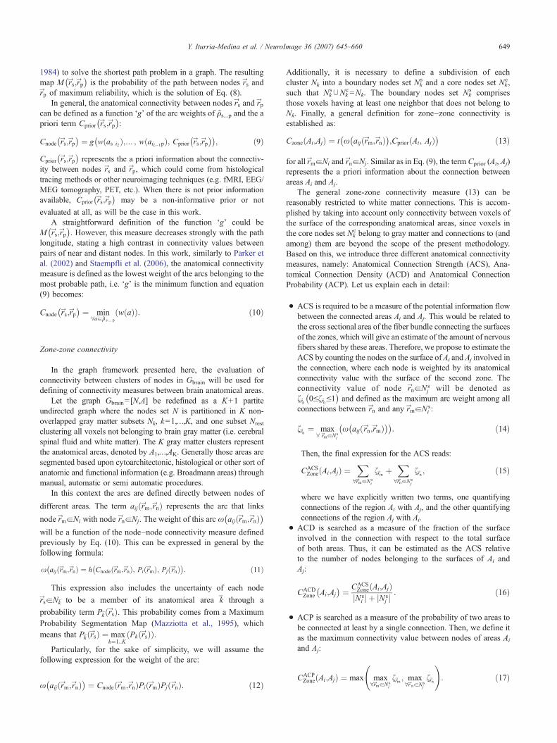
Fig. 4. Hypothetical simple 2D graph. The set of 36 nodes is consecutivelyenumerated, the nodes i1=11 and iq=25 in the figure are linked bytwo paths q1 rYi1 ;r
Yiq
� �and q2 rYi1 ;r
Yiq
� �. For path q1 rYi1 ;r
Yiq
� � ¼ u rYi1 ;rYi2ð Þ;f
u rYi2 ;rYi3ð Þ; N ;u rYiq�1 ;r
Yiq
� �g the sequence of nodes i1, i2, … , iq− 1, iq is 11,16, 15, 20, and 25. For q2 rYi1 ;r
Yiq
� �the sequence is: 11, 17, 22, 28, 33, 27, 32
and 25. The probability of path ρ2 is null, P[ρ2 (ri1, riq)]=0, because thispath has a curvature in node 33 that exceeds the critical angle /critical ¼
p2.
In particular / ¼ ar cosDrYi5 ;i6 ;Dr
Yi4 ;i5
jDrYi5 ;i6 jjDrYi4 ;i5 j !
¼ 3p4, where i4=28, i5=33 and
i6=27. In this case path ρ1 is more probable than ρ2.
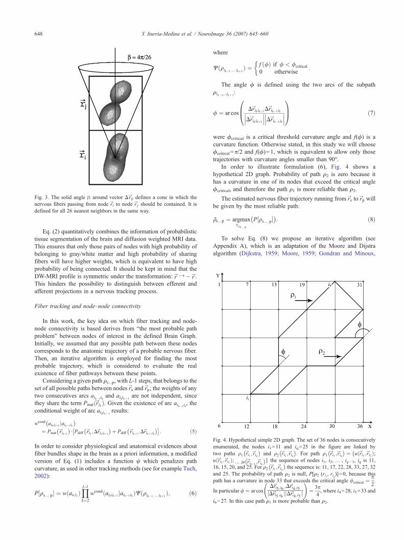
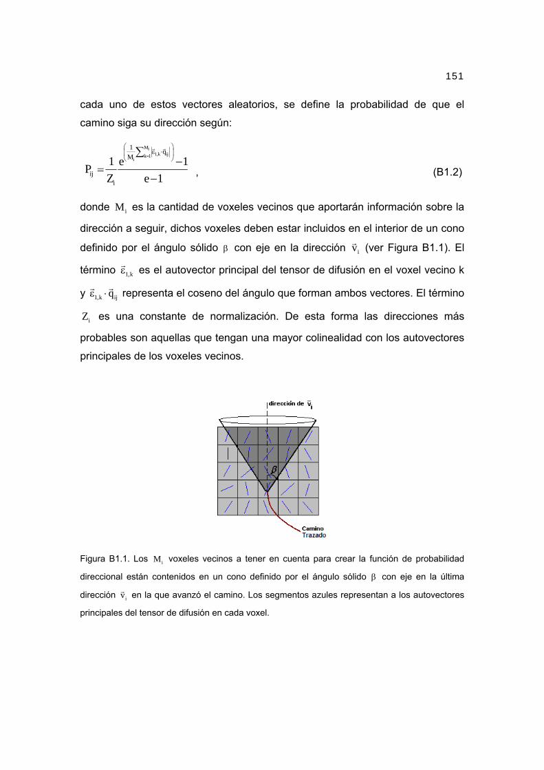
Fig. 3. The solid angle β around vector DrYij defines a cone in which thenervous fibers passing from node rYi to node rYj should be contained. It isdefined for all 26 nearest neighbors in the same way.
648 Y. Iturria-Medina et al. / NeuroImage 36 (2007) 645–660
Eq. (2) quantitatively combines the information of probabilistictissue segmentation of the brain and diffusion weighted MRI data.This ensures that only those pairs of nodes with high probability ofbelonging to gray/white matter and high probability of sharingfibers will have higher weights, which is equivalent to have highprobability of being connected. It should be kept in mind that theDW-MRI profile is symmetric under the transformation: rYY� rY.This hinders the possibility to distinguish between efferent andafferent projections in a nervous tracking process.
Fiber tracking and node–node connectivity
In this work, the key idea on which fiber tracking and node-node connectivity is based derives from “the most probable pathproblem” between nodes of interest in the defined Brain Graph.Initially, we assumed that any possible path between these nodescorresponds to the anatomic trajectory of a probable nervous fiber.Then, an iterative algorithm is employed for finding the mostprobable trajectory, which is considered to evaluate the realexistence of fiber pathways between these points.
Considering a given path ρs…p, with L-1 steps, that belongs to theset of all possible paths between nodes rYs and rYp; the weights of anytwo consecutives arcs aik −1ik and aikik + 1
are not independent, sincethey share the term Pmat rYikð Þ. Given the existence of arc aik −1ik, theconditional weight of arc aikik + 1
results:
wcond aik ikþ1 jaik�1 ik� �¼ Pmat rYikþ1
� �d Pdiff rYik ;Dr
Yik ikþ1
� �þ Pdiff rYikþ1;DrYikþ1 ik
� �� �: ð5Þ
In order to consider physiological and anatomical evidences aboutfiber bundles shape in the brain as a priori information, a modifiedversion of Eq. (1) includes a function ψ which penalizes pathcurvature, as used in other tracking methods (see for example Tuch,2002):
P½qs N p� ¼ wðas;i2ÞYL21k¼2
wcondðaik ikþ1 jaik�1ik ÞWðqik�1 N ikþ1Þ; ð6Þ
where
Wðqik�1 N ikþ1Þ ¼f ð/Þ if / < /critical
0 otherwise:
�
The angle ϕ is defined using the two arcs of the subpathρik −1…ik + 1
:
/ ¼ ar cosDrYik ikþ1Dr
Yik�1ikDrYik ikþ1DrYik�1ik
0B@
1CA ð7Þ
were ϕcritical is a critical threshold curvature angle and f(ϕ) is acurvature function. Otherwise stated, in this study we will chooseϕcritical =π/2 and f(ϕ)=1, which is equivalent to allow only thosetrajectories with curvature angles smaller than 90°.
In order to illustrate formulation (6), Fig. 4 shows ahypothetical 2D graph. Probability of path ρ2 is zero because ithas a curvature in one of its nodes that exceed the critical angleϕcritical, and therefore the path ρ1 is more reliable than ρ2.
The estimated nervous fiber trajectory running from rYs to rYp willbe given by the most reliable path:
qs N p ¼ argmax8qs N p
P½qs N p�� �
: ð8Þ
To solve Eq. (8) we propose an iterative algorithm (seeAppendix A), which is an adaptation of the Moore and Dijstraalgorithm (Dijkstra, 1959; Moore, 1959; Gondran and Minoux,
649Y. Iturria-Medina et al. / NeuroImage 36 (2007) 645–660
1984) to solve the shortest path problem in a graph. The resultingmap M rYs;rYp
� �is the probability of the path between nodes rYs and
rYp of maximum reliability, which is the solution of Eq. (8).In general, the anatomical connectivity between nodes rYs and rYp
can be defined as a function ‘g’ of the arc weights of ρs…p and the apriori term Cprior rYs;rYp
� �:
Cnode rYs;rYp� � ¼ g wðas i2Þ; N ; wðaiL�1pÞ; Cprior rYs;rYp
� �� �; ð9Þ
Cprior rYs;rYp� �
represents the a priori information about the connectiv-ity between nodes rYs and rYp, which could come from histologicaltracing methods or other neuroimaging techniques (e.g. fMRI, EEG/MEG tomography, PET, etc.). When there is not prior informationavailable, Cprior rYs;rYp
� �may be a non-informative prior or not
evaluated at all, as will be the case in this work.A straightforward definition of the function ‘g’ could be
M rYs;rYp� �
. However, this measure decreases strongly with the pathlongitude, stating a high contrast in connectivity values betweenpairs of near and distant nodes. In this work, similarly to Parker etal. (2002) and Staempfli et al. (2006), the anatomical connectivitymeasure is defined as the lowest weight of the arcs belonging to themost probable path, i.e. ‘g’ is the minimum function and equation(9) becomes:
Cnode rYs;rYp� � ¼ min
8aaq s N p
ðwðaÞÞ: ð10Þ
Zone-zone connectivity
In the graph framework presented here, the evaluation ofconnectivity between clusters of nodes in Gbrain will be used fordefining of connectivity measures between brain anatomical areas.
Let the graph Gbrain= [N,A] be redefined as a K+1 partiteundirected graph where the nodes set N is partitioned in K non-overlapped gray matter subsets Nk, k=1,…,K, and one subset Nrest
clustering all voxels not belonging to brain gray matter (i.e. cerebralspinal fluid and white matter). The K gray matter clusters representthe anatomical areas, denoted by A1,…,AK. Generally those areas aresegmented based upon cytoarchitectonic, histological or other sort ofanatomic and functional information (e.g. Broadmann areas) throughmanual, automatic or semi automatic procedures.
In this context the arcs are defined directly between nodes of
different areas. The term aij rYm;rYnð Þ represents the arc that links
node rYmaNi with node rYnaNj. The weight of this arc x aij rYm;rYnð Þ� �will be a function of the node–node connectivity measure definedpreviously by Eq. (10). This can be expressed in general by thefollowing formula:
x aij rYm;rYnð Þ ¼ h Cnode rYm;rYnð Þ; Pi rYmð Þ; Pj rYnð Þ� �
:� ð11Þ
This expression also includes the uncertainty of each node
rYsaNk to be a member of its anatomical area k through a
probability term Pk rYsð Þ. This probability comes from a MaximumProbability Segmentation Map (Mazziotta et al., 1995), whichmeans that Pk rYsð Þ ¼ max
k¼1::KPk rYsð Þð Þ.
Particularly, for the sake of simplicity, we will assume thefollowing expression for the weight of the arc:
Additionally, it is necessary to define a subdivision of eachcluster Nk into a boundary nodes set Nk
s and a core nodes set Nkc,
such that Nks∪Nk
c =Nk. The boundary nodes set Nks comprises
those voxels having at least one neighbor that does not belong toNk. Finally, a general definition for zone–zone connectivity isestablished as:
CzoneðAi;AjÞ ¼ t x aij rYm;rYnð Þ� �;CpriorðAi; AjÞ
� � ð13Þ
for all rYmaNi and rYnaNj. Similar as in Eq. (9), the termCprior (Ai, Aj)represents the a priori information about the connection betweenareas Ai and Aj.
The general zone-zone connectivity measure (13) can bereasonably restricted to white matter connections. This is accom-plished by taking into account only connectivity between voxels ofthe surface of the corresponding anatomical areas, since voxels inthe core nodes set Nk
c belong to gray matter and connections to (andamong) them are beyond the scope of the present methodology.Based on this, we introduce three different anatomical connectivitymeasures, namely: Anatomical Connection Strength (ACS), Ana-tomical Connection Density (ACD) and Anatomical ConnectionProbability (ACP). Let us explain each in detail:
• ACS is required to be a measure of the potential information flowbetween the connected areas Ai and Aj. This would be related tothe cross sectional area of the fiber bundle connecting the surfacesof the zones, which will give an estimate of the amount of nervousfibers shared by these areas. Therefore, we propose to estimate theACS by counting the nodes on the surface of Ai and Aj involved inthe connection, where each node is weighted by its anatomicalconnectivity value with the surface of the second zone. Theconnectivity value of node rYnaN s
j will be denoted asfYrn 0VfYrnV1� �
and defined as the maximum arc weight among allconnections between rYn and any rYmaN s
i :
fYrn ¼ max8 rYmaN s
i
x aij rYn;rYmð Þ� �� �: ð14Þ
Then, the final expression for the ACS reads:
CACSZoneðAi;AjÞ ¼
X8rYmaN s
i
fYrm þX8rYnaN s
j
fYrn ; ð15Þ
where we have explicitly written two terms, one quantifyingconnections of the region Ai with Aj, and the other quantifyingconnections of the region Aj with Ai.
• ACD is searched as a measure of the fraction of the surfaceinvolved in the connection with respect to the total surfaceof both areas. Thus, it can be estimated as the ACS relativeto the number of nodes belonging to the surfaces of Ai andAj:
CACDZone Ai;Aj
� � ¼ CACSZoneðAi;AjÞjN s
i j þ jN sj j
: ð16Þ
• ACP is searched as a measure of the probability of two areas tobe connected at least by a single connection. Then, we define itas the maximum connectivity value between nodes of areas Ai
and Aj:
CACPZoneðAi;AjÞ ¼ max max
8rYmaN si
fYrm ; max8rYnaN s
j
fYrn
!: ð17Þ
Fig. 5. Phantom tract configurations obtained from the Centre forNeuroimaging Sciences, Institute of Psychiatry, King's College London(http://neurology.iop.kcl.ac.uk/dtidataset/Common_DTI_Dataset.htm). Theconfigurations used in this study were: (a) straight crossing, (b) curvecrossing, and (c) tract inspired in the maple leaf (Feuille trajectory).
650 Y. Iturria-Medina et al. / NeuroImage 36 (2007) 645–660
Experimental data
Artificial dataDiffusion tensor phantom simulated data sets were obtained from
the Centre for Neuroimaging Sciences, Institute of Psychiatry,King's College London. The DW-MRI data were simulated using aspin-echo sequence with the following parameters: 30 diffusionencoding directions (Jones et al., 1999); b=1000 s/mm2; imageresolution 2×2×2 mm3; TE=160 ms. T2 values for the tract andbackground were assumed to be the same as white matter (65 ms)and grey matter (95 ms) at 1.5 T, respectively. Three data sets areavailable with varying levels of SNR (7, 15 and 31).
Three out of ten different tract configurations were selected toevaluate the performance of the proposed methodology (see Fig.5): straight crossing, curved crossing and the tract inspired in themaple leaf (Feuille trajectory). For each of them, the six diffusionelements, the eigenvectors and the corresponding T2-weightedimages for each SNR data set were provided. The correspondingODF maps were estimated using a simple procedure described inAppendix B. A threshold value was applied to the T2-weightedimage in order to create a binary mask (Pmat) expressing thepresence or not of gray/white matter tissue.
Additionally, two other artificial diffusion data sets werecreated using the following geometric parameters: 55×55×55voxels; image resolution 2×2×2 mm3. The first artificial data setrepresents a branching fiber tract (Fig. 6a). In branching areas, thefirst and second eigenvalues of the diffusion tensor were assumedto be equal (i.e. oblate tensor). The second artificial data setrepresents a fiber crossing of three orthogonal tracts (Fig. 6b). Incrossing areas, the three tensor's eigenvalues were assumed to beapproximately the same (i.e. spherical tensor). In both configura-tions, three different SNR (7, 15 and 31) were considered to createthe diffusion tensor elements. ODF maps were estimated using theprocedure described in Appendix B.
Human dataUsing a standard diffusion gradient direction scheme (twelve
diffusion-weighted images and a b=0 image), DW-MRI data wereacquired from 5 healthy subjects using a MRI scanner SiemensSymphony 1.5 T (Erlangen, Germany) and a single shot EPIsequence. To each subject, two interleaved sets of 25 slices of6 mm thickness with a distance factor of 100% were acquired withthe following parameters: b=1200 s/mm2; FOV=256×256 mm2;acquisition matrix=128×128; corresponding to an ‘in plane’spatial resolution of 2×2 mm2; TE/TR=160 ms/7000 ms. Twointerleaved sets were necessary because it was impossible to coverthe whole head with a good spatial resolution using a single set dueto a pulse sequence limitation (max: 35 slices). Both sets werejoined to form a volume of 50 contiguous slices of 3 mm thicknesscovering the whole brain for each subject. The aforementionedacquisition was repeated 5 times to improve signal to noise ratio(SNR). In order to improve EPI quality, magnitude and phasedifference images of a T2 gradient echo field mapping sequencewere acquired with TE=7.71 ms and 12.47 ms.
Also, a 3D high resolution T1-weighted image (MPRAGE)covering the whole brain was acquired with the followingparameters: 160 contiguous slices of 1 mm thickness in sagittalorientation; in plane FOV=256×256 mm2, corresponding to an inplane spatial resolution of 1×1 mm2; TE/TR=3.93 ms/3000 ms.
Although the scanner sequence performs an eddy currentautomatic correction, in order to remove remaining distortions an
affine 3D mutual normalized information-based registrationmethod (Studholme et al., 1998) was used. The DW-MRI imageswere attempted to be corrected from EPI distortions using the SPMFieldMap toolbox (Hutton et al., 2002).
T1-weighted 3D anatomical image was registered to the b=0image using a normalized mutual information method (Studholmeet al., 1998). Using the SPM2 toolbox (available at http://www.fil.ion.ucl.ac.uk/spm/software/spm2), a low dimensional normalization(Ashburner and Friston, 1999) to a stereotaxic space MNI (Evansand Collins, 1993) was estimated for the registered T1-weightedimage, which was written with an spatial resolution of2×2×2 mm3. Employing the aforementioned transformation,DW-MRI data were fitted to a diffusion tensor (Basser et al.,1994) in each voxel of the stereotaxic space. Tensors were rotated
Fig. 6. Additional artificial tract configurations created to explore theperformance of the proposed methodology. (a) Branching fiber tract. (b)Fiber crossing of three orthogonal tracts.
651Y. Iturria-Medina et al. / NeuroImage 36 (2007) 645–660
according to the method presented by Alexander and coworkers(Alexander et al., 2001).
Probabilistic tissues segmentations of gray matter, white matterand cerebral spinal fluid (Ashburner and Friston, 2000) wereobtained from the normalized T1-weigthed image using the SPM2toolbox. The gray and white matter segmentation probabilistic maps(PGM and PWM, respectively) were used to construct the anatomicalinformation function Pmat evaluating Eq. (3), with α=1. Also, thenormalized T1-weigthed image was automatically segmented into71 gray matter structures using the IBASPM toolbox (available athttp://www.fil.ion.ucl.ac.uk/spm/ext/#IBASPM) (Alemán-Gómez etal., 2006) and the average Probabilistic MRI Atlas created by theMontreal Neurological Institute (Collins et al., 1994; Evans et al.,1994). For evaluating the arcs weight in expression (11), theprobability of each voxel rYsaNk to belong to k-th anatomical areawas set to unity ðPk rYsð Þ ¼ 1Þ, although as it was mentioned inSection 2.4, this probability can be more realistically evaluatedemploying Maximum Probability Segmentation Maps (Mazziottaet al., 1995). Again, the ODF maps were estimated using theprocedure described in Appendix B.
Results
Artificial data
The performance of the proposed methodology was exploredusing artificial DW-MRI data. Firstly, anatomical connectionsbetween different regions of interest (ROIs), defined for thestraight crossing, curve crossing and Feuille trajectory wereestimated (see Fig. 7). Each ROI consists of seven contiguousvoxels representing a line perpendicular to the fiber tract beinganalyzed. Left column (Figs. 7a, c and e) shows the reconstructedconnection routes (most probable paths) between ROI1 and theothers, with SNR level of 15. These results illustrate the ability ofour method to reconstruct complex fiber tracts configurations (seefor example the Feuille trajectory results, Fig. 7e). Complementa-rily, right column (Figs. 7b, d and f) shows the correspondingmaximum voxel–voxel connectivity values with ROI1 (i.e. eachvoxel of the image volume was assigned its maximum voxel–voxelconnectivity value with the voxels of ROI1). Note that, althoughfor the straight crossing and curve crossing the method providesanatomical connection routes between ROI1 and ROI4, thecorresponding voxel–voxel connectivity values indicate the lowprobability of connection between these ROIs, which is inaccordance with the characteristics of the tracts configurations. Incontrast, the obtained voxel–voxel connectivity values betweenROI1–ROI2 and ROI1–ROI3 indicate the high probability ofconnection between these ROIs.
Secondly, we analyzed the branching configuration shown inFig. 6a. Both Fig. 8 and Table 1 show the results before and after ahypothetical loss of the white matter integrity. Three different ROIswere defined (Fig. 8a): ROI1 consists of two contiguous voxels atthe left end of the fiber tract, ROI2 consists of four contiguousvoxels at the upper right end of the tract and ROI3 is conformed bya single voxel at the bottom right end of the tract. For simulating ahypothetical loss of the white matter integrity (hereinafter, WM-affectation, for brevity), the values of two voxels in the binarymask (Pmat) were set to zero (each voxel located symmetrically atthe upper right tract or at the bottom right tract, see Fig. 8b). Figs.8c and d correspond to the maximum voxel–voxel connectivityvalues between the voxels of ROI1 and the rest of voxels beforeand after the WM-affectation, respectively. Also, Table 1 helps usto understand the interrelationship between the ACS, ACD andACP measures and their sensitivity to white matter affectation. Forexample, note that before WM-affectation the CZone
ACS (ROI1, ROI2)is around twice the CZone
ACS (ROI1, ROI3) since the total number ofsuperficial voxels in ROI1 and ROI2 duplicates the total number ofsuperficial voxels in ROI1 and ROI3 (i.e. 6 and 3 voxels,respectively). However, CZone
ACD (ROI1, ROI2) and CZoneACD (ROI1,
ROI3) are similar and the small difference between them can beexplained by the different geometrical characteristics of the definedROIs. In this case, both ROI2 and ROI3 present very highprobabilities of connection with ROI1 for all SNR levels. After theWM-affectation, these probabilities of connection as well as theACS and ACD measures decrease considerably.
Finally, the performance of our model in comparison with SLTand aFM methods was studied in the case of fiber crossing of threeorthogonal tracts, as shown in Fig. 9. Starting and ending ROIswere defined as planes of 5×5 voxels (i.e. each ROI containing 25voxels) at the two ends of the fiber tract being analyzed. Most ofthe fiber paths generated from ROI1 using SLT method terminatein the crossing fiber region or go to the perpendicular tracts (Fig.
Fig. 7. Resulting anatomical connections between different regions of interest (ROIs) defined for straight crossing, curve crossing and Feuille trajectory. Eachdefined ROI consists of seven contiguous voxels defining a perpendicular line to the corresponding fiber tract. Left column (Figs. 7a, c and e): reconstructedconnection routes (most probable paths) between ROI1 and the other defined ROIs, with SNR level of 15. Right column (Figs. 7b, d and f): correspondingmaximum voxel–voxel connectivity values between the image volume voxels and the ROI1 voxels. The color code represents the index of connectivity. (Forinterpretation of the references to colour in this figure legend, the reader is referred to the web version of this article.)
652 Y. Iturria-Medina et al. / NeuroImage 36 (2007) 645–660
9a). In contrast, both aFM and our graph-based tractographymethod reconstructed tracts between ROI1 and ROI2 (Figs. 9b andc, respectively). However, some fiber paths found by aFM failed tofollow the correct fiber tract (e.g. some of them strayed from thefiber tract being analyzed at the level of the crossing region, goingto the other perpendicular tracts and doing a U-turn before comingback to the main fiber to eventually reach the ending ROI).
Complementarily, Table 2 presents the obtained ACS, ACD andACP measures using aFM and the proposed approach. Notice thatalthough the zone–zone connectivity measures were not defined inthe aFM, we used the voxel–voxel connectivity provided by thismethod to evaluate Eqs. (15), (16) and (17). The resulting CZone
ACP
(ROI1, ROI2) using aFM is lower than that provided by ourapproach. Similarly, CZone
ACS (ROI1, ROI2) and CZoneACD (ROI1, ROI2)
measures for the aFM method are more distant from their idealvalues (50 for the ACS, and 1 for the ACD measure).
It is interesting to note that in this experiment, the fiber pathsobtained by our method look rougher or noisier (i.e. changingdirections from voxel to voxel) inside the crossing region (Fig. 9c).This effect is explained by the fact that in this region the diffusiontensor is nearly spherical, and any fiber tracking method relying onestimating an ODF will be affected by the goodness of this
estimation. In this work, the ODF is estimated from the Diffusiontensor model (Appendix B). This is a very simple method which isusually not able to describe complex fiber configurations, as is thecase in crossing regions. In the Summary and discussions sectionthe advantages of using more advanced models to infer the ODFwill be illustrated.
Human data
In order to explore the performance of the proposed method inreal data, we tried to replicate three well known brain anatomicalconnections. First, anatomical connections between voxels of theoccipital pole surfaces (OCCs) and voxels belonging to the whitematter and to the gray matter regions surfaces (WM-GMs) wereestimated. The reconstructed connection routes (most probablepaths) between left and right OCCs are shown in Fig. 10a. Figs. 10band c show axial maps of the node–node connectivity values at thelevel of the splenium of the corpus callosum and the lateralgeniculate nucleus, respectively. In these maps, each voxel wasassigned the maximum of all possible connectivity values between itand the voxels of both OCC areas. Fig. 10a illustrates how theconnection routes pass correctly through the splenium of the corpus
Fig. 8. Anatomical connections for the branching configuration before and after a hypothetical loss of the white matter integrity. (a) Three different ROIs weredefined: ROI1 consists of two contiguous voxels at the left end of the fiber tract, ROI2 consists of four contiguous voxels at the upper right end of the tract, andROI3 is conformed by a single voxel located at the bottom right end of the tract. Reconstructed connection routes (most probable paths) between ROI1–ROI2and ROI1–ROI3 are also represented. (b) To simulate a hypothetical loss of the white matter integrity, the values of two voxels in the binary mask (Pmat) were setto zero (each voxel located symmetrically at the upper right tract or at the bottom right tract). (c) Obtained maximum voxel–voxel connectivity values betweenthe image volume voxels and the ROI1 voxels before the hypothetical loss of the white matter integrity. The color code represents the index of connectivity. (d)Similar to (c), but after the hypothetical loss of the white matter integrity. (For interpretation of the references to colour in this figure legend, the reader is referredto the web version of this article.)
653Y. Iturria-Medina et al. / NeuroImage 36 (2007) 645–660
callosum and Figs. 10b and c confirm the expected high connectivityvalues for this region and the optic radiation, respectively. Theseresults are in accordance with existing anatomical knowledge(Gómez-Padrón et al., 1985; Witelson, 1989; Standring, 2004).
The anatomical connections between voxels of an axial seedplane (ASP) placed in the corticospinal tract at the level of the pons(which is considered as a region) and voxels belonging to theWM-GMs were also estimated. Fig. 10d shows the reconstructedroutes connecting the ASP and the left and right postcentrals gyrus,passing through the internal capsule. Moreover, Figs. 10e and fillustrate how regions of highest connectivity belong to the internalcapsule, the corona radiata and the motor cortex (Gómez-Padrón etal., 1985; Standring, 2004).
Table 1Results for branching configuration using the proposed connectivity graphmodel
Connectivity measures after affecting the white matter mask7 3.98 1.58 0.66 0.52 0.98 0.5915 3.96 1.57 0.66 0.52 0.99 0.5931 3.96 1.57 0.66 0.53 0.99 0.60
In a similar way, anatomical connections between voxels of themiddle frontal gyrus (MFGs) and the WM-GMs voxels wereestimated (see Figs. 10g–i). We tried to obtain the fibers trajectoriesfirst between the thalamus and the MFGs, and finally between theleft and right MFGs. In both cases, the main difficulty lies in the factthat the connecting fibers should pass through the crossing of threemajor bundles (i.e. intersection of the superior longitudinalfasciculus, the corona radiata and the corpus callosum). Note thatthe obtained routes connecting the thalamus and the MFGs (Fig.10g) pass through the internal capsule and the corona radiata inaccordance with previous anatomical studies (Gómez-Padrón et al.,1985; Standring, 2004). Also, those connection routes between theleft and right MFGs (Fig. 10g) pass specifically through the genuand the rostral body of the corpus callosum and Figs. 10h and iconfirm the expected high connectivity values for these regions,agreeing with Witelson's corpus callosum subdivision (Witelson,1989).
Fig. 11 shows the mean ACS, ACD and ACP maps between 71brain gray matter regions for five healthy subjects. For each subject,ACS, ACD and ACP measures were computed after eliminating notsignificant connectivity values between the WM-GMs voxels andthe set of defined gray matter structures. Significant values werefound by a z-test (H0: z≤0) with a 0.05 significance level. In eachmap, the element Ci,j is the mean connectivity value betweenregions i and j. Note that as we defined non-directed ACS, ACDand ACP measures, the resulting maps are symmetrical. Also, it canbe spotted 2 black lines (4 with the symmetry) in all maps. Thesecorrespond with the left and right subthalamic nucleus, which werenot correctly defined by the automatic parcellation method due totheir very small sizes.
Table 2Results for orthogonal crossing of three fiber tracts using aFM and theproposed connectivity graph model
Connectivity measures in orthogonal crossing using aFM and theconnectivity graph model
SNR aFM Graph model
CZoneACS CZone
ACD CZoneACP CZone
ACS CZoneACD CZone
ACP
654 Y. Iturria-Medina et al. / NeuroImage 36 (2007) 645–660
According to the mean ACS map (Fig. 11a), the precentralgyrus left and the postcentral gyrus left are the most connectedregions (i.e. they present the maximum ACS value, 387.16±97.87). These regions play an important role in a wide variety ofthe brain functions (e.g. motor and somatosensory functions). Ingeneral, frontal and temporal structures are the most connectedstructures. On the other hand, the most densely connected regionsare the caudate nucleus right and the thalamus right (connecting
Fig. 9. Tracking results for the fiber crossing of three orthogonal tracts withSNR level of 15. ROI1 and ROI2 were defined as planes of 5×5 voxels atthe two ends of the fiber tract being analyzed. (a) All paths generated fromROI1 using the SLT method. (b) Obtained connection routes between ROI1and ROI2 using the aFM method. (c) Obtained connection routes betweenROI1 and ROI2 using the proposed methodology.
around the 10±3% of their surfaces). It is known that the caudatenucleus is involved in the control of voluntary movement and inlearning and memory systems. Taking into account the mean ACPmap (Fig. 11c), the average connection density (i.e. the number ofall non-zero connections divided by the maximum possible numberof connections) was 0.7. This means that about the 70% of allpossible connections between any two of the defined brainstructures have a non-zero probability.
In order to evaluate (dis)similarity between the differentsubjects, correlation coefficients between their correspondingACS, ACD and ACP maps were estimated (see Table 3). Resultsshow significant correlations in all cases (the maximum p valueobtained was in the order of 10−209), supporting the hypothesis thathealthy subjects present similar ACS, ACD and ACP patterns forthe gray matter parcellation used in this study.
Summary and discussions
In this work, we developed a diffusion imaging methodologycapable to characterize anatomical connections between differentbrain gray matter structures. It consists of three basic steps: 1,definition of a Brain Graph model in which each voxel is consideredas a node of a non-directed weighted graph; 2, the use of an iterativealgorithm based on analysis of the voxels neighborhood to find theroute of maximum probability between two nodes and thesubsequent definition of the anatomical connectivity measurebetween them; 3, the definition of three anatomical connectivitymeasures between different gray matter regions, which areindividually considered as clusters of nodes in the graph.
In step 1, the probabilistic tissue segmentation of the anatomicalMR image and the intravoxel white matter orientational distribu-tion function (ODF), obtained from DW-MRI, are combined toestimate the probability of nervous fibers connection between twocontiguous nodes (voxels), which is associated to the weight of thearc connecting these nodes.
Generally, in the diffusion tracking framework, the fractionalanisotropy (FA) map is used to construct a binary mask which isemployed to constraint the fiber trajectories space (Conturo et al.,1999; Mori and van Zijl, 2002; Staempfli et al., 2006). Assumingthat nervous fibers are present only in those regions with highanisotropy, this mask is defined by an empirical threshold on the FAmap, which implies that regions where two or more fibers crosseach other will be ignored. To our knowledge, this work introducesfor the first time, the use of probabilistic brain tissue segmentationsof the anatomical MR images as a priori information to findanatomically plausible connection routes between any two voxels.
Fig. 10. (a) Obtained anatomical connection routes between the left and right occipital poles. Both thalami are represented as anatomical references. (b) Axialmap at the level of the splenium of the corpus callosum representing maximum voxel–voxel connectivity values between the WM-GMs voxels and the OCCsvoxels. (c) Axial map at the level of the lateral geniculate nucleus representing maximum voxel–voxel connectivity values between the WM-GMs voxels and theOCCs voxels. (d) Reconstructed connection routes between the ASP and the left and right postcentral gyrus. (e) Axial map representing maximum voxel–voxelconnectivity values between the WM-GMs voxels and the voxels of the ASP. (f) Coronal map representing maximum voxel–voxel connectivity values betweenthe WM-GMs and the ASP voxels. (g) Obtained connection routes among the left and right MFGs, and between each MFGs and the ipsilateral thalamus. (h)Coronal map representing maximum voxel–voxel connectivity values between the WM-GMs voxels and the MFGs voxels. (i) Inter-hemispheric planerepresenting maximum voxel–voxel connectivity values between the WM-GMs voxels and the MFGs voxels. In (b), (c), (e), (f), (h) and (i) the color coderepresents the index of connectivity. Each connectivity map was overlaid on the corresponding T1-weighted image. (For interpretation of the references to colourin this figure legend, the reader is referred to the web version of this article.)
655Y. Iturria-Medina et al. / NeuroImage 36 (2007) 645–660
Additionally, we allow for tuning the relative importance betweenthe probabilistic gray and white matter segmentations through the αparameter (see Eq. (3)). For α≥1, the segmentation of white matterwill have equal or bigger weight than the gray matter segmentation,which agrees with the fact that nervous fibers are mostly in thewhite matter. However, α should not be considerably greater thanone (for example: α=10), because voxel–voxel connections aroundgray matter can be rejected. Thus, although in this study we choseα=1, the appropriate selection of this parameter requires detailedfuture analysis.
On the other hand, the weight of the arc connecting twoneighboring nodes is defined by taking into account the fiberscoherence along its direction. The probability that a fiber is present
around a particular arc is evaluated by computing the integral ofthe ODF in a solid angle along its direction (see Fig. 3), whichcontributes to reduce discretization errors at the same time thatcomplex structural fiber distributions can be considered. However,the ODF is just one of several measures that implicitly reflect fibercoherence. In this sense, the graph-based approach has theadvantage that other functions can be used for this purpose, suchas those characterizing fiber distribution with various maxima oforientation (Jansons and Alexander, 2003; Tuch, 2004; Alexander,2005) or even the ellipsoids given by the diffusion tensors (Basseret al., 1994).
In order to find the anatomical connection route between twonodes in the defined Brain Graph, we explored the set of all
Table 3Correlations between the ACS, ACD and ACP maps of the 5 subjects
For each connectivity measure, the elements above the main diagonal are thecorrelation coefficients.All the correlations are significant; the maximum p value obtained was in theorder of 10−209.
Fig. 11. Mean connectivity results for 71 gray matter regions defined on thebrain of five healthy subjects: (a) ACS, (b) ACD and (c) ACP. In each map,the element Ci,j is the mean connectivity across subjects between regions iand j. The color code represents the index of connectivity.
656 Y. Iturria-Medina et al. / NeuroImage 36 (2007) 645–660
possible discrete paths to select the route which optimize certainfunction designed according to physiological criteria. A similarexample of this type of procedure are the Fast Marching (FM)tractography techniques (Parker et al., 2002; Staempfli et al.,2006), in which the route connecting two voxels should minimizethe “time” necessary to arrive from one voxel to the other. In our
case, the fiber tractography is expressed in terms of the mostprobable path in the defined Brain Graph. Figs. 7–9 illustrate theperformance of the proposed tractography method in the artificialDW-MRI data. The results show that the methodology we haveintroduced here is able to reconstruct correctly complex fiberconfigurations such as straight crossing, curve crossing, Feuilletrajectory, branching tract and orthogonal crossing of three tracts.Also, the obtained connection routes between the left and rightOCCs (Fig. 10a), the defined ASP and both postcentral gyrus (Fig.10d), the thalamus and left and right MFGs (Fig. 10g) werepresented. These results agree with existing anatomical knowledge(Gómez-Padrón et al., 1985; Witelson, 1989; Standring, 2004).
Quantification of the anatomical connectivity between twovoxels can be defined according to the parameters of the connectionroute among them and also taking into account the a prioriinformation about the connectivity between these voxels, whichcould come from previous anatomical and functional studiesbased on histological tracing methods or neuroimaging techniques(e.g. fMRI, EEG/MEG tomography, PET, etc.). This allows theintegration between different anatomical and functional connec-tivity measures. In this work, similar to Parker et al. (2002) andStaempfli et al. (2006), an anatomical connectivity measure isdefined as the lowest weight of the arcs set belonging to the mostprobable path. However, we consider that other node–node(voxel–voxel) connectivity measures should be explored.
To characterize anatomical connections between K brain graymatter structures, the previous Brain Graph was redefined as aK+1 partite graph by partitioning the initial nodes set in K non-overlapped gray matter subsets and one subset clustering theremaining nodes. Based on the latter, three connectivity measureswere defined: Anatomical Connection Strength (ACS), AnatomicalConnection Density (ACD) and Anatomical Connection Prob-ability (ACP). ACS provides an estimation of the potentialinformation flow between any pair of regions. It is considered
657Y. Iturria-Medina et al. / NeuroImage 36 (2007) 645–660
proportional to the amount of nervous fibers shared by theseregions. To estimate it we considered that, similar as in a system oftubes in which the liquids flow in one extreme of a specific tubedepends on its cross section area and on the rate of liquids, thepotential nervous information flow can be reflected by the crosssection area of the fiber connector volume on the surfaces of thetwo regions. Here, the ACS is estimated by counting the“effective” number of nodes on the surfaces of the zones involvedin the connection, where each node is counted according to afunction which represents its anatomical connectivity value withthe surface of the second zone (this function ranges between 0, noconnected, and 1, completely connected). When the zones ofinterest present a high number of superficial nodes, the proposedACS estimation has the inconvenient that, even if the superficialnodes of the zones are not well connected, the accumulation of agreat number of small node–node connectivity values can cause ahigh ACS. To avoid this, it is reasonable to eliminate those node–node connections with values below a specified threshold beforecomputing the ACS, which also contributes to eliminate thenuisance connections. Although in this work we used a z-test inorder to eliminate non-significance connectivity values betweenthe WM-GMs voxels and the set of defined gray matter structures,the selection of the threshold could be carried out using moreadvanced local and global thresholding models, such as local falsediscovery rate technique (Efron, 2004, 2005) or image thresholdingbased on the EM algorithm (Yakoub et al., 2006). This will be thesubject of future work.
On the other hand, ACD is a measure of the fraction of theconnected superficial nodes with respect to the total number ofsuperficial nodes of both areas. It permits, for example, to know if apair of zones has more or less density of connection than other pairof zones with different or equal number of superficial nodes. Tworegions with a high ACS value (compared with the ACS betweenothers pairs of regions) not necessarily have to present a high ACDvalue. This situation could take place when two regions of interestcontain a high number of superficial nodes. Similarly, a pair ofzones with a low ACS value can present a high ACD value, whichoccurs specifically when the zones contain a small number ofsuperficial nodes (each node having an anatomical connectivityvalue close to 1 with the surface of the other zone).
While ACS and ACD quantify the strength and density of thepossible connection respectively, ACP measures the maximumprobability of two regions to be connected at least by a singleconnection. It allows to infer if any two gray matter regions can befunctionally related independently of the strength and density ofthe possible connection. Additionally, other zone–zone connectiv-ity measures can be defined and some of them could be directlyformulated as the combination of the three proposed measures.
Fig. 11 show the mean maps of ACS, ACD and ACP obtainedbetween 71 gray matter structures for five healthy subjects.Significant correlations among the connectivity matrixes of thedifferent subjects were found (Table 3), which could support thehypothesis that healthy subjects present similar ACS, ACD andACP patterns for the used gray matter parcellation. Beforepresenting the aforementioned results, the anatomical connectionsobtained for the branching configuration before and after ahypothetical loss of the white matter integrity were presented(Fig. 8 and Table 1), illustrating how the ACS, ACD and ACPmeasures reflect the white matter affectation. In a similar way,more detailed comparisons between normal and pathological ACS,ACD and ACP maps (or its combinations) could be a potential
procedure to detect and diagnose pathologies causing functionalcognitive deficiencies related to white matter injury, such as:Alzheimer, Schizophrenia and Dyslexia. Compared to connectivitymaps of normal subjects, abnormal ones can reveal certain damagein the anatomical interconnectivity between multiple functionalcognitive brain areas, allowing to find those regions that are notwired properly. Other possible application of the aforementionedconnectivity maps is to use them as a priori or complementaryinformation in brain functional connectivity studies (see forexample Sotero et al., 2007).
However, the lack of information about the direction of nervousfibers in DW-MRI data hinders the possibility of distinguishingbetween efferent and afferent projections. Thus, in the defined non-directed weighted graph, the direction of the arcs (distinctionbetween initial and terminal nodes) is irrelevant and making themeasures ACS, ACD and ACP to be bidirectional. This constitutesan inherent important limitation of DW-MRI techniques. Never-theless, in a previous work (Young, 1993) a connectivity matrix ofthe primate cerebral cortex was reported where approximately onlythe 15% of the total possible connections between 73 brain areaswere not reciprocals.
An important element in the Brain Graph model is the voxelsize of the MR images (1/resolution). Reduction of the voxel size(which can be achieved directly in the data acquisition) implies amore accurate description of the brain structure, i.e. a bettercharacterization of the intravoxel anisotropy as well as a morereliable tissue segmentation. However, the decrease of the voxelsize leads to a worse SNR and implies an increase in thecomputational cost of the methodology.
Other important element is the angular resolution of thediffusion weighted images. In this work, we have achievedcompetitive results with the use of low angular resolution data,but certainly a better performance of the methodology can beobtained using high angular resolution techniques, for example Q-ball Imaging (Tuch, 2004) and diffusion spectrum MRI (Wedeen etal., 2005). A better estimation of the ODF implies a precisecharacterization of the intravoxel white matter disposition and thusan accurate evaluation of the fibers coherence along arcs direction,which subsequently implies a more realistic characterization of thebrain structure. In order to illustrate this, in Fig. 12 a comparison ofthe fiber crossing of three orthogonal tracts using the introducedgraph-based tractography with ODF maps estimated from (a) theDiffusion tensor model (same results that in Fig. 9c) and (b) the Q-ball Imaging technique (Tuch, 2004) is shown. Close-ups of thefiber crossing region are shown, illustrating that the calculatedroutes using the Diffusion tensor model (Fig. 12a) are considerablyrougher or noisier than those routes obtained using the Q-ballImaging technique (Fig. 12b). This supports the idea that highangular resolution-based techniques allow to get better results.
The Graph Theory constitutes an ideal framework for modelingdiverse system situations. Given the wide use of the graphframework in several areas of physics and mathematics, multipleproblems and practical applications have been undergone. In thisstudy, this framework is applied for the first time to the fiber trackingproblem and to the subsequent quantification of the brain anatomicalconnections from DW-MRI data. However, open problems remainrelated to the recognition of false fiber trajectories and to the cor-responding elimination of nuisance connections. Statistical models, inwhich a relative high number of subjects should be considered, can beuseful to investigate the variability of the connectivity maps in order toeliminate non-significant and superfluous connections. Also, as was
Fig. 12. Comparison of the fiber crossing of three orthogonal tracts using the graph-based tractography method with SNR level of 15 and ODF maps estimatedaccording to: (a) Diffusion tensor model, (b) Q-ball Imaging technique. Close-ups of the fiber crossing region are shown.
658 Y. Iturria-Medina et al. / NeuroImage 36 (2007) 645–660
mentioned in Section 2.4, the probability that a node belongs to agiven gray matter structure can be specified employing MaximumProbability Segmentation Maps or even using Spatial ProbabilisticAnatomical Maps (Mazziotta et al., 1995). In the future, moreadvanced graph models should be able to employ both thisprobability and the uncertainty in the estimation of the fiberorientation distribution function. This, in turn, could be used toestimate the error associated to arc weights, node–node and zone–zone connectivity measures. Additionally, future studies in animalsshould be addressed to further testing of the performance of theproposed methodology.
Acknowledgments
Authors would like to thank Nelson Rubal Lorenzo, AgustínLage-Castellanos and Erick C. Jones for their useful comments onthe anatomical, statistical and algorithmic aspects of this work,respectively. Also, we thank to Roberto C. Sotero and ThomasKoenig, for the final revision of the manuscript.
Appendix A. Algorithm to solve the most probable pathproblem
Given a Brain Graph Gbrain= [N,A], let us define some quan-tities before setting up the algorithm:
|N|: Cardinality of the set N, i.e. the number of elementsbelonging to set N.
N− s: Set of nodes that belong to Gbrain except node ‘s’,N�s ¼ N=frYsg.MðrYvÞ: Map of probabilities of the path between node ‘s’ and allnodes rYvaN�s,MðrYvÞ ¼ P qðrYs;rYvÞ½ � and MðrYsÞ ¼ 1.Ni
neig: Nearest neighborhood of the i-th node.
This algorithm proceeds in |N|−1 iterations as follows:
a) Set initially:
a.1) S=N− s
a.2)MðrYiÞ ¼
1; rYi ¼ rYs;wðasiÞ; rYia N neig
i0; otherwise:
8<:
a.3) qðrYs;rYiÞ ¼ asi; 8rYiaN neigs
b) Find rYjaS such that MðrYjÞ ¼ max8rYiaS
MðrYiÞb.1) Set a new SpS=frYjgb.2) If S =Ø, then Stop; else continue
c) For all rYmaN neigj and rYmaS, set
c.1) qðrYs; rYmÞ ¼ q rYs; rYj
� � [ ajm� �
;
c.2) If P q rYs; rYmð Þ½ � > MðrYmÞ thenqðrYs; rYmÞ ¼ qðrYs; rYmÞ; MðrYmÞ ¼ P½qðrYs; rYmÞ�
c.3) go to b.
659Y. Iturria-Medina et al. / NeuroImage 36 (2007) 645–660
Finally, the map MðrYpÞ for rYpaN�s represents the finalprobability of the path of maximum reliability according to Eq.(8) between nodes rYs and rYp denoted by qðrYs; rYpÞ.
Appendix B. White matter orientational distribution function
The intravoxel white matter orientational distribution function(ODF) Ψ ( u) is defined as the radial projection of the probabilitydensity function (PDF) PðRYÞ (Wedeen et al., 2005):
wð uÞ ¼Zþl0
R2Pð uRÞdR; ðB1Þ
being û a unitary vector and RY ¼ uR the relative spin
displacement.Considering the PDF for anisotropic Gaussian diffusion:
P RY �
¼ ð4ptÞ�3=2ðjDjÞ�1=2e�RY T
D�1RY4t ; ðB2Þ
Then, substituting in Eq. (B1) and using the identity:Zþl0
xmeax2dx ¼
C ðmþ1Þ2
�2a
mþ12
; ðB3Þ
where Γ is the Gamma function, we can obtain the ODF as:
w uð Þ ¼ 1C
uTD�1 u� ��3
2 ðB4Þ
Here, C is a normalization constant which ensures that the ODFis properly normalized to unit mass.
References
Alemán-Gómez, Y., Melie-García, L., Valdes-Hernández, P., 2006.IBASPM: Toolbox for automatic parcellation of brain structures.Presented at the 12th Annual Meeting of the Organization for Hum.Brain Mapp., June 11–15, 2006, Florence, Italy. Available on CD-Romin NeuroImage, Vol. 27, No.1.
Alexander, D.C., 2005. Multiple-fiber reconstruction algorithms fordiffusion MRI. Ann. N. Y. Acad. Sci. 1064, 113–133.
Basser, P.J., Pajevic, S., 2000. Statistical artifacts in diffusion tensor MRI(DT-MRI) caused by background noise. Magn. Reson. Med. 44, 41–50.
Basser, P.J., Mattiello, J., LeBihan, D., 1994. Estimation of the effective self-diffusion tensor from the NMR spin echo. J. Magn. Reson., Ser. B. 103,247–254.
Basser, P.J., Pajevic, S., Pierpaoli, C., Duda, J., Aldroubi, A., 2000. In vivofiber tractography using DT-MRI data. Magn. Reson. Med. 44,625–632.
Behrens, T.E., Johansen-Berg, H., Woolrich, M.W., Smith, S.M., Wheeler-Kingshott, C.A., Boulby, P.A., Barker, G.J., Sillery, E.L., Sheehan, K.,Ciccarelli, O., Thompson, A.J., Brady, J.M., Matthews, P.M., 2003.Non-invasive mapping of connections between human thalamus andcortex using diffusion imaging. Nat. Neurosci. 6, 750–757.
Collins, D.L., Neelin, P., Peters, T.M., Evans, A.C., 1994. Automatic 3Dintersubject registration of MR volumetric data in standardized Talairachspace. J. Comput. Assist. Tomogr. 18, 192–205.
neuronal fiber pathways in the living human brain. Proc. Natl. Acad. Sci.U. S. A. 96, 10422–10427.
Dijkstra, E.W., 1959. A note on two problems in connexion with graphs.Numer. Math. 269–271.
Efron, B., 2004. Large-scale simultaneous hypothesis testing: the choice of anull hypothesis. J. Am. Stat. Assoc. 99, 96–104.
Efron, B., 2005. Local false discovery rates. http://www-stat.stanford.edu/∼brad/papers/.
Evans, A.C., Collins, D.L., 1993. A 305-member MRI-based stereotacticatlas for CBF activation studies. Proceedings of the 40th AnnualMeeting of the Society for Nuclear Medicine.
Evans, A.C., Collins, D.L., Neelin, P., MacDonald, D., Kamber, M., Marrett,T.S., 1994. Three-dimensional correlative imaging: applications inhuman brain mapping. In: Thatcher, R.W., Hallett, M., Zeffiro, T., John,E.R., Huerta, M. (Eds.), Functional Neuroimaging. Technical Founda-tions, pp. 145–162.
Gómez-Padrón, I., Silva Loynaz, C., Seuc Chiu, A., 1985. Anatomía II.Folleto complementario. Ministerio de salud pública, Cuba.
Gondran, M., Minoux, M., 1984. Graphs and Algorithms. John Wiley andSons Ltd., Chichester.
Hagmann, P., Thiran, J.P., Jonasson, L., Vandergheynst, P., Clarke, S.,Maeder, P., Meuli, R., 2003. DTI mapping of human brain connectivity:statistical fibre tracking and virtual dissection. NeuroImage 19,545–554.
Hagmann, P., Kurant, M., Gigandet, X., Thiran, P., Wedeen, V.J., Meuli, R.,Thiran, J.P., 2006. Imaging the brain neuronal network with diffusionMRI: a way to understand its global architecture. Proc. ISMRM 436.
Hutton, C., Bork, A., Josephs, O., Deichmann, R., Ashburner, J., Turner, R.,2002. Image distortion correction in fMRI: a quantitative evaluation.NeuroImage 16, 217–240.
Iturria-Medina, Y., Valdes-Hernandez, P., Canales-Rodriguez, E., 2005.Measures of anatomical connectivity obtained from neuro diffusionimages. Available on CD-Rom in NeuroImage, Vol. 26, No.1; Presentedat the 11th Annual Meeting of the Organization for Hum. Brain Mapp.,June 12–16, 2005, Toronto, Ontario, Canada.
Jones, D.K., Horsfield, M.A., Simmons, A., 1999. Optimal strategies formeasuring diffusion in anisotropic systems by magnetic resonanceimaging. Magn. Reson. Med. 42, 515–525.
Jun Zhang, Hao Ji, Ning Kang and Ning Cao, 2005. Fiber Tractography inDiffusion Tensor Magnetic Resonance Imaging: A Survey and Beyond.Technical Report No. 437-05 ed., Department of Computer Science;University of Kentucky; Lexington; KY.
Koch, M.A., Norris, D.G., Hund-Georgiadis, M., 2002. An investigation offunctional and anatomical connectivity using magnetic resonanceimaging. NeuroImage 16, 241–250.
Mazziotta, J.C., Toga, A.W., Evans, A., Fox, P., Lancaster, J., 1995. Aprobabilistic atlas of the human brain: theory and rationale for itsdevelopment. The International Consortium for Brain Mapping (ICBM).NeuroImage 2, 89–101.
Moore, E.F., 1959. The Shortest Path Through a Maze. Harvard UniversityPress, Cambridge, Massachusetts, pp. 285–292.
660 Y. Iturria-Medina et al. / NeuroImage 36 (2007) 645–660
Mori, S., van Zijl, P.C., 2002. Fiber tracking: principles and strategies—Atechnical review. NMR Biomed. 15, 468–480.
Mori, S., Crain, B.J., Chacko, V.P., van Zijl, P.C., 1999. Three-dimensionaltracking of axonal projections in the brain by magnetic resonanceimaging. Ann. Neurol. 45, 265–269.
Parker, G.J., Alexander, D.C., 2003. Probabilistic Monte Carlo basedmapping of cerebral connections utilising whole-brain crossing fibreinformation. Inf. Process. Med. Imag. 18, 684–695.
Parker, G.J., Haroon, H.A., Wheeler-Kingshott, C.A., 2003. A frameworkfor a streamline-based probabilistic index of connectivity (PICo) using astructural interpretation of MRI diffusion measurements. J. Magn.Reson. Imaging 18, 242–254.
Ramnani, N., Behrens, T.E., Penny, W., Matthews, P.M., 2004. Newapproaches for exploring anatomical and functional connectivity in thehuman brain. Biol. Psychiatry 56, 613–619.
Sporns, O., Tononi, G., Kotter, R., 2005. The human connectome: astructural description of the human brain. PLoS. Comput. Biol. 1,e42.
Staempfli, P., Jaermann, T., Crelier, G.R., Kollias, S., Valavanis, A.,Boesiger, P., 2006. Resolving fiber crossing using advanced fast
marching tractography based on diffusion tensor imaging. NeuroImage30, 110–120.
Standring, S., 2004. Gray's Anatomy: The Anatomical Basis of Medicineand Surgery, 39th edition. Churchill Livingstone.
Studholme, Hill, Hawkes, 1998. A normalized entropy measure of 3-Dmedical alignment. Proc. Med. Imaging, vol. 3338. SPIE Press, SanDiego, CA, pp. 132–143.
Tench, C.R., Morgan, P.S., Blumhardt, L.D., Constantinescu, C., 2002.Improved white matter fiber tracking using stochastic labeling. Magn.Reson. Med. 48, 677–683.
Weinstein, D., Kindlmann, G., Lundberg, E., 1999. Tensorlines: advection-diffusion based propagation through diffusion tensor fields. Proc. IEEEVisualization, San Francisco, CA, pp. 249–253.
Witelson, S.F., 1989. Hand and sex differences in the isthmus and genu ofthe human corpus callosum. A postmortem morphological study. Brain112 (Pt. 3), 799–835.
Yakoub, B., Lorenzo, B., Farid, M., 2006. Image thresholding based on theEM algorithm and the generalized Gaussian distribution. PatternRecogn. 40, 619–634.
Young, M.P., 1993. The organization of neural systems in the primatecerebral cortex. Proc. Biol. Sci. 252, 13–18.
57
3.2. ARTÍCULO 2
Yasser Iturria-Medina, Roberto C. Sotero, Erick J. Canales-Rodríguez, Yasser
Alemán-Gómez and Lester Melie-García, 2008. Studying the Human Brain
Anatomical Network via Diffusion-Weighted MRI and Graph Theory. Neuroimage,
40, 1064-1076.
www.elsevier.com/locate/ynimg
NeuroImage 40 (2008) 1064–1076
Studying the human brain anatomical network via diffusion-weightedMRI and Graph Theory
Yasser Iturria-Medina,a,⁎ Roberto C. Sotero,b Erick J. Canales-Rodríguez,a
Yasser Alemán-Gómez,a and Lester Melie-Garcíaa
aNeuroimaging Department, Cuban Neuroscience Center, Avenue 25, Esq 158, #15202, PO Box 6412, Cubanacán, Playa, Havana, CubabBrain Dynamics Department, Cuban Neuroscience Center, Havana, Cuba
Received 20 June 2007; revised 18 October 2007; accepted 30 October 2007Available online 19 November 2007
The brain is one of the most challenging systems found in nature.It can be viewed as a complex network consisting of highlyinterconnected processing regions. Its response to any external
stimulus relies on the cooperation among these specialized centers,which can be classified according to their anatomical and functionalproperties (Brodmann, 1909; Mazziotta et al., 1995; Toga et al.,2006; Mountcastle, 2007). Thus, the study of their anatomical andfunctional connectivity constitutes an indispensable step towards theunderstanding of the brain specialization and integration (Sporns etal., 2005).
Previous works in mammalian species (i.e. cat and macaquemonkey) have shown that cortical anatomical connection matrices,obtained post-mortem, exhibit “small-world” attributes (Spornsand Zwi, 2004; Hilgetag and Kaiser, 2004). That is, anatomicalbrain connection patterns are characterized by a high clusteringindex and a short average distance between any two regions.Small-world topology is generally associated with global and localparallel information processing, sparse connectivity between nodesand low wiring costs (Bassett and Bullmore, 2006). Using thissame connectivity datasets, structural and functional motifscomposition (characteristic network building blocks) were studied(Sporns and Kotter, 2004). The results supported the hypothesisthat while brain networks maximize both the number and thediversity of functional motifs, the repertoire of structural motifs isrelatively small.
Functional human brain networks derived from functionalMagnetic Resonance Imaging (fMRI), Electroencephalogram(EEG) and Magnetoencephalographic (MEG) data also exhibitsmall-world properties (Stam, 2004; Eguiluz et al., 2005; Salvadoret al., 2005; Achard et al., 2006; Bassett et al., 2006). However,characteristics of the human brain anatomical network have beenpoorly investigated. This is due to difficulties in defining the basicstructural elements of the human brain in terms of nodes andconnections (Sporns et al., 2005) and also because the commoninvasive tracer methods cannot be applied. Recent steps in thatdirection were given by He et al. (2007), which investigatedanatomical connections patterns in the human cerebral cortex invivo using cortical thickness measurements from magneticresonance images. For this, the cerebral cortex was segmentedinto 54 different areas for 124 normal brains, and any two areas
1065Y. Iturria-Medina et al. / NeuroImage 40 (2008) 1064–1076
were considered anatomically connected if they had statisticallysignificant correlations in cortical thickness. This is based onstudies suggesting that interregional statistical associations incortical thickness provide important connectivity information(Worsley et al., 2005; Lerch et al., 2006). Then, a threshold valuewas applied to interregional correlation matrix in order to constructa binary undirected graph and estimate its properties, principallysmall-world properties and the connectivity degree distribution.Their results supported the hypothesis that human brain anatomicalnetworks present small-world attributes and follow a degreedistribution characterized by an exponentially truncated power-law.However, as their approach was limited to cortical networks,important subcortical structures such as the thalamus or the amygdales,which keep vital connections with cortical areas, were not taken intoaccount.
On the other hand, the development of diffusion-weightedMagnetic Resonance Imaging (DW-MRI) techniques in the lastdecade makes possible the noninvasive study of the anatomicalcircuitry of the living human brain (Mori et al., 1999; Conturo etal., 1999; Tuch, 2002; Parker et al., 2002; Koch et al., 2002;Behrens et al., 2003; Hagmann et al., 2006; Iturria-Medina et al.,2007). In this context, Hagmann et al. (2006) reported for the firsttime small-world attributes in networks of small human corticalareas estimated from DW-MRI techniques. In that study, nodes ofthe analyzed network corresponded to small cubic regions ofinterest (ROI) covering the gray matter tissue, while arc weightswere assigned according to the estimated fiber densities betweennodes, which had been previously computed using an in vivoprobabilistic nervous fiber tracking procedure (Wedeen et al.,2005). By applying a threshold to the created graph, anunweighted version was constructed and its small-world andhierarchical properties were analyzed. Their results show similarsmall-world topologies to those obtained for the rat and macaquemonkey brain networks, which were created using post-mortemtracing techniques.
In the present paper we continue the characterization of thehuman brain anatomical connections by extending previous worksin several ways. First, instead of an unweighted graph as inHagmann et al. (2006) and He et al. (2007), a weighted version willbe used for modeling the brain anatomical network. In thisapproach, the weights are obtained from the anatomical connectionsprobability (ACP) matrix which gives the probability that any twoareas are connected at least by a single nervous fiber. For obtainingthe ACP matrix, anatomical connections patterns between 90different anatomical gray matter regions will be estimated usingDW-MRI techniques and Graph Theory (Iturria-Medina et al.,2007). These regions include both cortical and subcortical structuresas defined by Tzourio-Mazoyer et al. (2002) according to functionaland anatomical criteria. Finally, in addition to previous small-worldand degree distribution analysis, other important network proper-ties, such as efficiency, vulnerability, betweenness centrality andmotif composition will be investigated.
The remainder of the paper is organized as follows. In theMaterials and methods section the DW-MRI methodology used forestimating brain anatomical connections is briefly described, and itis shown that the obtained anatomical network can be viewed as aweighted non-directed graph. After that, concepts like small-worldand network efficiency, degree distribution, vulnerability, between-ness centrality and motifs composition are briefly exposed. Theexperimental data and its preprocessing are also described. In theResults section significant findings are presented. Finally, the last
section summarizes and discusses the principal results, andproposes some open problems to be considered in future studies.
Materials and methods
Mapping zone-zone brain anatomical connections using DW-MRI
DW-MRI techniques have being widely used to estimate thenervous fiber pathways connecting brain regions of interest (Moriet al., 1999; Conturo et al., 1999; Tuch, 2002; Parker et al., 2002;Koch et al., 2002; Behrens et al., 2003; Hagmann et al., 2006;Iturria-Medina et al., 2007). Recently, a novel DW-MRI and GraphTheory methodology (Iturria-Medina et al., 2007) was introducedwith the principal purpose of summarizing anatomical connectionspatterns between brain gray matter areas. The proposed procedureconsists of three major steps:
1. The cerebral volume is represented as a non-directed weightedgraph Gbrain,0= [N0, A0, W0], where N0 is the set of voxels(nodes) having a non-zero probability of belonging to somecerebral tissue, A0 is the set of white matter links (arcs) betweencontiguous voxels in N0, and W0 is a set of real numbersrepresenting arcs weights. The weight of an arc is chosen so thatit represents the probability that contiguous linked nodes arereally connected by nervous fibers. It is defined by taken intoaccount both the probability that linked nodes belong to gray/white matter (evaluated according to the probabilistic tissuessegmentation of the corresponding anatomic T1-weightedimage) and the probability of nervous fibers to be orientedaround the direction of the arc (evaluated using the intravoxelwhite matter Orientational Distribution Function [ODF] esti-mated via DW-MRI techniques) (see Eq. (A1)). This ensuresthat only those pairs of contiguous nodes with high probabilityof belonging to gray/white matter and high probability ofsharing fibers will have high arc weights, which is equivalent tohave high probability of being connected. Also, since the DW-MRI profile is symmetric (efferent and afferent projections cannot be distinguished) Gbrain,0 is modeled as a non-directed graph(i.e. distinction between initial and terminal arc nodes isirrelevant).
2. In this step, an iterative algorithm (see Appendix C) is employedfor finding the most probable trajectory (see Eq. ((A6)) betweenany two nodes, which is assumed to be the hypothetical nervousfiber pathway running between these points. Thus, quantifica-tion of the anatomical connectivity between both points iscarried out according to the intrinsic information of thisestimated connection route. Specifically, the node-node anato-mical connectivity measure (ranging between 0, not connected,and 1, perfectly connected) is defined as the lowest weight of thearcs set belonging to the most probable path (see Eq. (A7)). Thisensures that only those brain points with high arc weights(probability of white matter connection) of all the arcs belongingto their connection route will have a high connectivity value.
3. In order to characterize anatomical connections between n braingray matter structures, the previous graph Gbrain,0 is redefined asa n+1 partite graph Gbrain by partitioning the initial nodes set N0
into n non-overlapped gray matter subsets and one subsetclustering the remaining nodes. In this context, the new weightednon-directed brain graph Gbrain= [N, A,W] consist of a set N of nnodes (gray matter regions), a set A of arcs (direct white matterconnections between gray matter regions) and a set W of arc
1066 Y. Iturria-Medina et al. / NeuroImage 40 (2008) 1064–1076
weights (probability of connections between the gray matterregions). Graphically, Gbrain is a discrete set of points (nodes)representing anatomic regions and a set of lines without arrow(arcs) representing connections between the regions. Based onthe latter, three connectivity measures were defined: AnatomicalConnection Strength (ACS), Anatomical Connection Density(ACD) and Anatomical Connection Probability (ACP). Theinterpretation of these measures is as follows. ACS provides anestimation of the potential information flow between any pairof regions, which is considered proportional to the amount ofnervous fibers shared by these regions. As an indicator of thelatter, we took the cross section area of the fiber connectorvolume on the surfaces of the two regions. This is estimated bycounting the “effective” number of nodes on the surfaces of thezones involved in the connection, where each node is countedaccording to its maximum probability of being connected withthe nodes in the surface of the second zone (see Eq. (A8)). Onthe other hand, ACD is a measure of the fraction of theconnected superficial nodes with respect to the total number ofsuperficial nodes of both areas (see Eq. (A10)). It allows, forexample, to know if a pair of zones has more or lessconnection density than other pair of zones with different orequal number of superficial nodes. Finally, ACP measures themaximum probability of any two regions to be connected atleast by a single nervous fiber connection. It is estimated as themaximum connectivity value between the superficial nodes ofboth involved areas (see Eq. (A11)) and allows to infer if anytwo gray matter regions can be functionally related indepen-dently of the strength and density of their possible anatomicalconnection.
In the present study, as our goal is to analyze a map of possiblebrain anatomical connections implying potential functional inter-change between gray matter areas (i.e. which areas are directlyconnected or not), we employ the ACP measure for weightingzone-zone connections in Gbrain. Further works might include ACSand ACD measures in order to complement the description of thebrain anatomical network.
Graph analysis to characterize brain anatomical connections
A great number of natural systems can be represented bycomplex networks. Graph Theory is usually considered the mostappropriate framework for the mathematical treatment of complexnetworks. In general, a complex network can be represented as agraph in which nodes correspond to the elements of the system andarcs to the interactions between them (Boccaletti et al., 2006). Inour specific case, we want to study the weighted brain networkGbrain= [N, A,W], which model the anatomical connections between90 cortical and subcortical gray matter regions. Gbrain will becharacterized attending to six basic aspects: small-world, networkefficiency, degree distribution, vulnerability, betweenness centralityand motifs composition.
Small-world and network efficiency
The concept of “small-world” is strongly related to the averageshortest path length (L) and clustering coefficient (C) concepts. Letus explain these in detail: the average shortest path length (L) of agiven graph G=[N, A,W], is a measure of the typical separationbetween two nodes i and j (8i, jaN), and it is defined as the mean
of geodesic lengths dij over all pairs of nodes (Watts and Strogatz,1998; Watts, 1999; Boccaletti et al., 2006):
L ¼ 1nðn� 1Þ
Xi;jaG
ipj
dij ð1Þ
In the unweighted network context (wij= [0,1]aℕ), thegeodesic length dij is defined as the number of arcs along theshortest path connecting nodes i and j. In the case of weightednetworks (wijaℝ), the path with the minimum number of nodes isnot necessarily the optimal dij and in some cases it is necessary todefine a physical length associated to each arc (this should be afunction of the characteristics of the hypothetical link among anynodes i and j). In this work, we follow the suggestion of Boccalettiet al. (2006), and assume that the physical length of an arcconnecting nodes i and j is inversely proportional to the probability
of the analyzed connection, i.e. lij ¼ 1wij
. That is, as the probability
of nervous fiber connection is lower the nodes are more distant.Note that this assumption do not penalizes arc length according tothe real spatial separation between the position of the modeled graymatter regions or according to the longitude of the connecting fiberpathway. This is because the defined probability of nervous fiberconnection only depends on the “diffusion data coherence” and thewhite/gray matter presence along the estimated connection routes,and not on its longitude. Thus, long range connections (such asthose maintained by the optic radiation and the occipital–frontalfascicule) can have arc length values similar to short rangeconnections, only depending of their corresponding connectionprobabilities. The geodesic length dij is finally defined as thesmallest sum of the arc lengths throughout all the possible pathsfrom node i to node j. Note that for the particular case ofunweighted graphs, lij=1 for all arcs and the geodesic lengths dijreduces to the minimum number of arcs traversed to get from i to j.
On the other hand, the clustering coefficient is a measure of theinherent tendency to cluster nodes into strictly connectedneighborhoods (Watts and Strogatz, 1998). In a weighted graph,the clustering around a node i can be calculated as the geometricaverage of subgraph node weights (Onnela et al., 2005):
Ci ¼ 1kiðki � 1Þ
Xj;kaGj;kpi
wijd wjkd wki
� �13; ð2Þ
where ki is the number of arcs connecting node i (named degree ofthe node i) and the weights are scaled by the largest weight in the
network, wij ¼ wij
maxðwijÞ. The clustering coefficient for the whole
graph G is defined as the average of clustering around each node(Watts and Strogatz, 1998):
C ¼ 1n
XiaG
Ci: ð3Þ
Formally, Watts and Strogatz (1998) defined small-world net-works as those having small average shortest path length, like random
networks (kuLreal
Lrandf1), and high clustering coefficient, much larger
than random networks (guCreal
CrandH1). Additionally, the small-
worldness condition lies in satisfying that rug
kN1 (Humphries et
al., 2006).
1067Y. Iturria-Medina et al. / NeuroImage 40 (2008) 1064–1076
The concept of small-world has been also expressed in terms ofthe information flow (Latora and Marchiori, 2001). That is, small-world networks are very efficient in terms of global and localcommunication (they have high global and local efficiency Eglob
and Eloc, respectively). The Eglob of a graph G is defined as:
Eglob ¼ 1nðn� 1Þ
Xi;jaG
ipj
1dij
: ð4Þ
This measure reflects how efficiently information can beexchanged over the network, considering a parallel system inwhich each node sends information concurrently along thenetwork. On the other hand, the Eloc of G is defined as theaverage efficiency of the local subgraphs:
Eloc ¼ 1n
XiaG
Eglob Gið Þ; ð5Þ
where Gi is the subgraph of the neighbors of i. This measurereveals how much the system is fault tolerant, showing howefficient the communication is among the first neighbors of i whenit is removed. That is, the efficiency formalization gives a clearphysical meaning to the concept of small-world, and allows aprecise quantitative analysis of weighted networks (Latora andMarchiori, 2001).
In order to compare the efficiency of a given real network withthe efficiency of its equivalent random network (characterized bythe same number of nodes and arcs placed randomly), from now onwe will refer to the relative local efficiency (Eloc∗ ) and the relativeglobal efficiency (Eglob∗ ) measures (i.e. the ratio between thelocal and global efficiencies of the real and random networksrespectively).
Degree distribution
Since not all nodes in a complex network have the same degree,usually a degree distribution P(k) is defined. This gives theprobability that a randomly selected node has k arcs (Erdös andRényi, 1959). The degree distribution properties are commonlyemployed to classify networks into different categories. Amaral etal. (2000) presented evidences of the occurrence of three classes ofsmall-world networks attending to their degree distributionproperties: 1) scale-free networks, 2) broad-scale networks, and3) single-scale networks.
Scale-free networks, for example the World-Wide Web (Albertet al., 1999), are characterized by a degree distribution that decaysas a power law, i.e. P(k)~k−α, with exponents varying in the range2bαb3. This power law indicates the preferential attachment ofthe nodes in the network to some specific hub nodes.
Broad-scale networks are characterized by a degree distribu-tion that has a power law regime followed by a sharp cutoff, i.e.P(k)~kα−1f(k/kcrit). The function f(k/kcrit) has a sharp cut-off fordegrees kNkcrit, constraining the number of nodes that can beconnected to the hub nodes.
Finally, single-scale networks are characterized by a degreedistribution with a fast decaying tail, i.e. P(k)~ f(k/kcrit). Commonlyfor single-scale and broad-scale regime the sharp cutoff functionsf(k/kcrit) are exponential or Gaussian (Amaral et al., 2000).
The information expressed by the degree distribution func-tion is often presented by the cumulative degree distribution
PcðkÞ ¼Pl
k V¼k Pðk VÞ, which is usually used to reduce the effectsof noise corresponding to small networks (Strogatz, 2001; Heet al., 2007).
Vulnerability
The vulnerability analysis of complex networks providesvaluable quantitative information about the possible damagecaused by the hypothetical failure of its elements. That is, thistype of analysis allows to identify which are the most critical orindispensable structures for the appropriate operation of thenetwork, and in the specific case of brain networks, it could beuseful to evaluate the damage caused by illness known to affectgray matter connections such as Alzheimer Disease (Pearson etal., 1985; Morrison et al., 1986) and Schizophrenia (Mitelmanet al., 2007).
By associating the performance of a network with its globalefficiency, the vulnerability Vi of a node i can be defined as thedrop in network performance when node i and its connections areremoved (Newman and Park, 2003; Goldshtein et al., 2004; L.da F.Costa et al., 2006):
Vi ¼Eglob � Ei
glob
Eglob; ð6Þ
where Eglob and Eglobi are the global efficiency of the network with
and without node i.Then, the vulnerability of the entire network G is defined as the
maximum vulnerability for all of its nodes (Latora and Marchiori,2005; L.da F.Costa et al., 2006):
V ¼ maxi
Vi: ð7Þ
Betweenness centrality
Betweenness centrality is a widely used measure to identify themost central nodes in a graph, which are associated to those nodesthat acts as bridges between the others nodes (Freeman, 1977;Dall'Asta et al., 2006; Bassett et al., 2006; Honey et al., 2007). It isdefined as the fraction of shortest paths between pairs of nodes thatpasses through a given node. Mathematically, for weightednetworks, if σkj
w is the total number of shortest paths from k to jand σkj
w(i) is the number of these paths passing through node i, theweighted betweenness centrality of node i is (Dall'Asta et al., 2006):
bwi ¼X
k;jaGkpj
rwkjðiÞrwkj
: ð8Þ
Motifs composition
Network motifs are subgraphs that appear more frequently in areal network than could be statistically expected, and are associatedto the network evolution (Milos et al., 2002; Sporns and Kotter,2004; Onnela et al., 2005). To detect those motifs that are likely to beimportant, Milos et al. (2002) proposed to compare the analyzed realnetwork to suitably randomized networks and to select patternsappearing in the real network at numbers significantly higher thanthose in the randomized networks. Different motifs classes are
1068 Y. Iturria-Medina et al. / NeuroImage 40 (2008) 1064–1076
generally distinguished according to the motif's size (M), represent-ing the number of involved nodes, and the number and pattern ofinterconnections.
In the case of weighted networks, Onnela et al. (2005) definedthe intensity (IM) of motif M as the geometric mean of its arcweights, and the coherence (QM) of motif M as the ratio of thegeometric to the corresponding arithmetic mean. Based on thesemeasures, motif scores were defined as:
ZIM ¼ IM � hiM ið Þhi2M i � hiM i2� �1
2
;
ZQM ¼ QM � hqM ið Þhq2M i � hqM i2� �
12
;
ð9Þ
where ZIM and ZQM are the motif intensity and coherence scorerespectively; iM and qM are the total intensity and coherence ofmotif M in one realization of the random regime, respectively.
Experimental data
DW-MRI datasets corresponding to 20 right-handed healthysubjects (mean age: 31.10, S.D.: 7.43) were acquired using a MRIscanner Siemens Symphony 1.5 T (Erlangen, Germany) and asingle shot EPI sequence. Each dataset consists of 12 diffusion-weighted images and a b=0 image, with the following parameters:50 contiguous slices of 3 mm thickness; b=1200 s/mm2 for theweighted images; FOV=256×256 mm2; acquisition matrix=128×128; corresponding to an ‘in plane’ spatial resolution of2×2 mm2; TE/TR=160 ms/7000 ms. The aforementionedacquisition was repeated 5 times to improve signal to noise ratio(SNR). In order to improve EPI quality, magnitude and phasedifference images of a T2 gradient echo field mapping sequencewere acquired with TE=7.71 ms and 12.47 ms. Also, for eachsubject a 3D high resolution T1-weighted image (MPRAGE)covering the whole brain was acquired with the followingparameters: 160 contiguous slices of 1 mm thickness in sagittalorientation; in plane FOV=256×256 mm2, corresponding to an inplane spatial resolution of 1×1 mm2; TE/TR=3.93 ms/3000 ms.
In order to remove remaining distortions an affine 3D mutualnormalized information-based registration method (Studholme etal., 1998) was used. The DW-MRI images were corrected fromEPI distortions using the SPM FieldMap toolbox (Hutton et al.,2002). The T1-weighted 3D anatomical image was registered tothe b=0 image using a normalized mutual information method(Studholme et al., 1998). Both diffusion-weighted images and T1-weighted images were interpolated and written with a spatialresolution of 2×2×2 mm3. The registered interpolated T1-weighted image was automatically segmented into 90 gray matterstructures (Tzourio-Mazoyer et al., 2002) using the IBASPMtoolbox (available at http://www.fil.ion.ucl.ac.uk/spm/ext/#23IBASPM) (Alemán-Gómez et al., 2006). ODF maps wereestimated using the procedure described in Appendix B.
Additionally, a set of three brain anatomical connectivitymatrices were obtained from the Computational CognitiveNeuroscience Laboratory, Indiana University Bloomington (http://www.indiana.edu/~cortex/CCNL.html). These datasets correspondto the cat cerebral cortex, the macaque monkey visual cortex and themacaque monkey cerebral cortex, and consist of unweightedmatrices with number of nodes 95, 30 and 73, respectively.
In all cases, randomized counterpart versions of the originalnetworks were created using a rewiring algorithm (Maslov andSneppen, 2002). This algorithm preserves the degree of eachindividual node, but connection weights are randomized untilweight correlations with the original network are lost.
Results
Fiber tracking and zone–zone connectivity
Using the DW-MRI methodology described above, anatomicalconnections between the defined 90 brain gray matter structureswere estimated for the 20 healthy subjects. Fig. 1 presents theobtained mean intersubject ACP matrix. The element Cij is theconnectivity value between regions i and j. As previouslymentioned, this map is symmetric. Self connections are excluded,which implies a diagonal black line in the matrix. Also, it shouldbe kept in mind that for each subject the anatomical reconstructionconsisted of the whole brain with the two hemispheres (i.e.including callosal connections). Note for example the highconnectivity values between the left and right superior frontalgyrus, or between the left and right superior occipital poles, whichis in accordance with existing anatomical knowledge (Gómez-Padrón et al., 1985; Witelson, 1989; Standring, 2004).
In order to evaluate intersubject dis(similarity), correlationscoefficients between their corresponding ACP matrices werecalculated. Significant correlations coefficients were obtained(ranging between 0.65 and 0.88) with corresponding p values inthe order of 10−220.
Small-world and network efficiency analysis
First, the relative clustering coefficient γ, the relative averageshortest path length λ and the small-worldness parameter σ werecalculated for each subject. The results (first three columns ofTable 1) confirm the expected small-world attributes of the studiedbrain anatomical networks according to the Watts-Strogatz (1998)and Humphries et al. (2006) conditions (i.e. λ~1, γH1 and σN1).The obtained mean parameters of interest were γmean=1.85,λmean=1.12 and σmean=1.64, satisfying the previous conditions.
In a second statistical analysis, a network efficiency studyrevealed that, compared with the corresponding random networks,the human brain architectural network (as well as other mammalianspecies brain networks, as we will see later) presents smaller globalefficiency and bigger local efficiency, i.e. both individual andmean values of Eglob∗ are under 1, while the corresponding Eloc∗values are always above 1 (see columns 4 and 5 of Table 1,respectively). These results are in accordance with those obtainedfor brain functional networks corresponding to the same graymatter parcellation scheme (Achard and Bullmore, 2007). In theSummary and discussion section we will comment more aboutthis, including the analysis of other mammalian brain speciesresults.
Degree distribution analysis
A degree distribution analysis revealed that the studied brainanatomical networks correspond to a power law regime followedby a sharp cutoff, as broad-scale networks. Table 1 (columns 6and 7) presents the obtained α and kcrit parameters correspondingto a broad-scale regime following the form P(k)~kα−1 exp(k/k crit).
Fig. 1. Mean ACP matrix for 90 gray matter regions defined on the brain of 20 healthy subjects. The element Ci,j is the connectivity value between regions i andj. Self connections are excluded, which implies a diagonal black line in the matrix. As previously mentioned, this map is symmetric. The color code represents theindex of connectivity.
1069Y. Iturria-Medina et al. / NeuroImage 40 (2008) 1064–1076
Fig. 2 illustrates the inter-subject mean cumulative degreedistribution and its standard deviation. All the correspondingmultiple determination coefficients, R-square (i.e. a measure ofhow successful the fit is in explaining the variation of the data, avalue closer to 1 indicates a better fit), were in the order of 0.99.The mean estimated exponent α was 1.34. Additionally, theresulting mean parameter kcrit indicate that even the mostconnected areas in the brain have a physical constraint of around5.81 inter-regional connections according to the used gray matterparcellation. These results are similar to those reported in Achardet al. (2006) for a human functional network involving the samegray matter areas (i.e. a degree distribution followed anexponentially truncated power law with an exponent parameterα=1.80 and a cutoff degree kcrit=5).
Vulnerability and betweenness centrality analysis
In order to make a first inference about the most critical orindispensable structures in the brain anatomical networks, thevulnerability of the 90 defined brain gray matter areas for eachsubject were computed using expression (6). Fig. 3a summarizesthe obtained mean vulnerability results. The identified mostvulnerable areas are: putamens, precuneus, insulas, superiorparietals and superior frontals. In a complementary analysis, thebetweenness centrality of each gray matter area was estimatedusing expression (8). The identified most central areas agree totallywith the obtained in the previous vulnerability analysis (see Fig.3b). In both cases, the selected regions were identified by applyinga z-test (H0: z=0) with a 0.05 significance level to the resulting
1070 Y. Iturria-Medina et al. / NeuroImage 40 (2008) 1064–1076
mean vulnerability and mean betweenness centrality vectorsrespectively.
Motifs composition
Since the human brain anatomical networks studied here aresymmetrical, our motifs composition analysis was restricted to findonly those symmetrical motifs that appear significantly increasedin the analyzed networks (let us say motifs with identity number[ID] 9 and 13 for motifs of size 3, and motifs with ID 75, 95, 159,178, 194 and 199 for motifs of size 4; see Fig. 4a). In order to carryout the motifs analysis, 30 reference random matrices weregenerated. Fig. 4b and c show the obtained motifs intensity andmotifs coherence scores for each subject, with motifs sizes 3 and 4,respectively. Notice that for M=3 (Fig. 4b), only a candidate motifwith ID=13 seems to appear significantly increased while forM=4(Fig. 4c) candidate motifs with ID=159, 194 and 199 are those thatseem to appear significantly increased. Using a 0.05 significancelevel, we confirmed that the mentioned candidate motifs showstatistically significant intensity and coherence deviation from thereference system, being them the obtained symmetrical humanbrain motifs of size 3 and 4.
Summary and discussion
In this work some basic statistical aspects of the human brainanatomical network were analyzed. The studied networks consistedof white matter connections between 90 cortical and subcortical graymatter regions, which were defined according to functional andanatomical criterions (Tzourio-Mazoyer et al., 2002). Connectionsamong the different regions were estimated for 20 healthy subjectsaccording to a graph-based DW-MRI procedure (Iturria-Medina etal., 2007) and the weighted networks analysis was centered in theirsmall-world attributes, efficiency, degree distribution, vulnerability,betweenness centrality and motifs composition properties.
To our knowledge, until now only two previous works havebeing presented with a similar purpose. In the first previous study(Hagmann et al., 2006), the analyzed brain network consisted of alot of gray matter cubic regions defining nodes whose correspond-ing arc weights connections were assigned according to theestimated nervous fiber density (Hagmann et al., 2004) betweenthem. An unweighted version of the created graph was analyzedtaking into account its small-world and hierarchical properties. Inthe second previous study (He et al., 2007), the networksummarized the obtained connectivity patterns between 54 corticalareas segmented for 124 normal brains. Connections between areaswere estimated using cortical thickness measurements frommagnetic resonance images. The brain anatomical unweightednetwork analysis was centered principally in its small-worldattributes and degree distribution properties.
In our first brain anatomical network statistical analysis, small-world and efficiency properties were studied. The results confirmthe small-world attributes of the human brain anatomical network(Table 1). The obtained mean parameters of interest wereγmean=1.85, λmean=1.12, with a resulting small-worldness para-meter of σmean=1.64, satisfying the Watts-Strogatz (1998) andHumphries et al. (2006) conditions (i.e. λ~1, γH1 and σN1).However, it is important to notice that according to Hagmann etal. (2006), small-worldness parameter as well as the relativeclustering coefficient should increases significantly when thenumber of brain network nodes increases. Although our resultsare in agreement with the results reported by Hagmann et al.(2006) and He et al. (2007) it should be noted that the used graymatter parcellation procedures differ in these studies. Addition-ally, our analysis was based on a weighted network scheme incontrast to an unweighted scheme as in previous works.Unfortunately, these procedure differences hinder a reliablequantitative parameter comparison between these three humananatomical studies.
Other brain mammalian species (cat and macaque monkey)present similar small-world anatomical attributes (Sporns and Zwi,2004; Hilgetag and Kaiser, 2004). Nevertheless, as happens withprevious human studies, a quantitative parameters comparisonbetween our results and the reported by these post-mortem tracinganimal studies it is not straightforward due to differences in theemployed procedures (mainly the different used gray mattersegmentation schemes).
In addition, the network efficiency analysis provided aninteresting result: compared with the corresponding randomnetworks, human brain anatomical networks present bigger localefficiency and smaller global efficiency. These results agree withthat obtained by Achard and Bullmore (2007) for human brainfunctional networks, and also with those obtained by us for the catcerebral cortex (Eloc∗ =1.37 and Eglob∗ =0.96), the macaque monkeyvisual cortex (Eloc∗ =1.24 and Eglob∗ =0.97) and the macaquemonkey cerebral cortex (Eloc∗ =1.86 and Eglob∗ =0.93). In ouropinion, this suggests that mammalian brains evolved trying tomaintain a high local efficiency, which is equivalent to prioritizethe integration among regions specialized in similar types offunctional information and, also, guaranties the tolerance topossible fails at the local level. On the other hand, the globalefficiency (i.e. the capacity to exchange information among all theregions) is small compared with corresponding random networks.A reason for this could be that the global exchange may not becompletely necessary, a fact related to the optimization of the brainintegration process.
Fig. 2. Estimated inter-subject mean cumulative degree distribution (red points) and standard deviation (blue error bars). The green line represents the fittedexponential truncated power law corresponding to a broad scale regime of the form P(k)∼kα−1exp(k/kcrit), with α=1.34 and kcrit =5.81. Inset: log–log plot of themean cumulative degree distribution. The red points indicate observed data, the blue line is the best fitted exponential truncated power law (RBS=0.9987), thegreen line is an exponential (Rexp=0.9942), and the orange line is a power law (RSF=0.8005).
1071Y. Iturria-Medina et al. / NeuroImage 40 (2008) 1064–1076
A degree distribution analysis revealed that the studied brainnetworks present a power-law regime followed by a sharp cutoff(Fig. 2), as broad-scale networks. In this kind of networks, thepreferential attachment to the hub nodes has a physical constraint,which in terms of brain anatomical connections is related to themaximum number of areas connected to the hub nodes andresponds to structural cost optimization process (e.g. optimizationof the axonal volume covering inter-regional brain connections). Inaddition, other anatomical and functional human brain studies havepresented similar degree distribution results (Achard et al., 2006;He et al., 2007). This supports the broad-scale attributes of thehuman brain network; however, final conclusions about this topicrequire future analysis to much larger brain networks withthousands of nodes.
The vulnerability and betweenness centrality analysis allowedidentifying the most critical anatomical nodes in the brain, revelingquantitative information about the global damage caused by thehypothetical failure of these nodes. According to the gray matterparcellation that was used, the most vulnerable and central areaswere (see Fig. 3): putamens, precuneus, insulas, superior parietalsand superior frontals. On the other hand, note that some areas causea negative vulnerability to the studied brain networks, which meansthat the anatomical brain system can be more efficient withoutthem (the most representative are: superior temporal poles,pallidums, supramarginals and hechls). This can be related to theanatomical cost of their existence, and suggest that even implying apossible loss in global anatomical efficiency, these structures were
maintained in the brain circuitry through the evolutionaryprocesses due to their specific important functions. Also, as aninteresting point, we may have expected that thalamic regionsbelong to the most critical or indispensable gray matter centers inthe brain. However, the used vulnerability and betweennesscentrality measures are strongly related to the number ofconnections of the analyzed areas, and the obtained results indicatethat thalamic regions are not the most connected areas althoughsurely they have important connections with some specificanatomic regions.
In the context of brain networks, a structural (anatomical) motifmay consist of a set of brain areas and pathways that can bepotentially engage in different patterns of interactions (Sporns andKotter, 2004). In practice, networks motifs are identified as thosesubgraphs appearing more frequently in a real network than couldbe statically expected (Milos et al., 2002; Onnela et al., 2005). Inthis work, it was looked for the first time into the structural motifcomposition of the human brain anatomical network. According tothe used gray matter parcellation and the employed weighted motifdetection procedures (Onnela et al., 2005), the obtained structuralmotifs were those with ID=13, for M=3, and with ID=159, 194and 199, for M=4 (see Fig. 4). This result keeps some essentialsimilarities with the obtained for cat and macaque cerebral cortexby Sporns and Kotter (2004), that is: motifs at M=4 are theexpanded versions of the obtained motif at M=3, forming areciprocally connected nodes chain, where pairs of connectionslinking the ends of the chain can be absent; thus, nodes in the
Fig. 3. Mean inter-subject vulnerability (a) and betweennes centrality (b) results for the 90 defined brain gray matter areas. Additionally, using a z-test (H0: z=0)with a 0.05 significance level, the most vulnerable and central areas were identified. In both cases, these areas are: putamens, precuneus, insulas, superiorparietals, and superior frontals.
1072 Y. Iturria-Medina et al. / NeuroImage 40 (2008) 1064–1076
motifs are highly integrated with their neighbors although some ofthem do not communicate directly, reflecting the basic principles ofintegration and segregation in the brain.
A limitation of the presented study is the symmetricalconfiguration of the analyzed brain connectivity matrices, whichis a consequence of the inherent symmetrical properties of DW-MRI techniques (distinction between afferent and efferent fiberprojections it is not possible yet). This fact causes, for example, therestriction of the motif composition analysis to consider only thosesymmetrical candidate motifs. Nevertheless, a previous work(Young, 1993) reported that around 85% of the total possibleconnections between 73 primate brain areas are reciprocals.
An important element in the DW-MRI Graph-Based methodol-ogy employed here for estimating brain anatomical connections(Iturria-Medina et al., 2007) is the angular resolution of thediffusion-weighted images. In this work we used low angularresolution data due to a system limitation, but certainly more
reliable results can be obtained using high angular resolutiontechniques, which allows a more precise characterization of theintravoxel white matter orientation (Tuch, 2004; Wedeen et al.,2005) and thus a more realistic characterization of the brainstructure. Other relevant matter is how to use the obtained ACPmatrices to elucidate which gray matter areas are actuallyconnected or not. A tentative alternative could be the selection ofa threshold value to create unweighted connectivity matrices.However, the choice of the appropriate threshold is generally anelusive point, and that's why in this study we chose to work onlywith probability of connections between zones instead of thesimpler on–off connectivity analysis. Additionally, future worksmight be directed to explore the effects of different trackingmethods on the network attributes. Surely, common findings acrossdifferent tracking methods would provide more confidence for theanatomical network graphical description. Nonetheless, in recentstudies (unconcluded) we have obtained significant similarity
Fig. 4. Motifs results for motifs size M=3 and M=4. (a) Candidate symmetrical motifs of size 3 and 4. Numbers refer to the motif's identity number (ID). (b)Obtained motifs intensity and motifs coherence scores for each subject, with M=3. (c) Obtained motifs intensity and motifs coherence scores for each subject,withM=4. In panels (b) and (c), the color code represents the z-score index. Using a 0.05 significance level, significant motifs found in the analyzed human brainnetworks were those with ID=13, for M=3, and with ID=159, 194 and 199, for M=4.
1073Y. Iturria-Medina et al. / NeuroImage 40 (2008) 1064–1076
among the connectivity patterns of healthy subjects using twodifferent fiber tractography procedures (i.e. the Graph-basedmethod employed here and the probabilistic tracking methodimplemented in the FSL software package [http://www.fmrib.ox.ac.uk/fsl]). This will be the subject of a separate publication.
Reliable gray matter parcellation is crucial for obtainingconsistent connectivity patterns between individuals. Therefore, akey element of the used methodology to create the brainanatomical network is its high dependency on the employed atlas.Although the atlas used here was carefully created taking intoaccount relevant anatomical and functional details (Tzourio-Mazoyer et al., 2002), in the future it might be more meaningful
to use advanced integrative atlases based on finer cytoarchitecture,myeloarchitecture and MRI procedures (Toga et al., 2006; He etal., 2007).
Further studies should focus on: improving the characteriza-tion of the brain anatomical connections (using for examplehigh angular resolution DW-MRI techniques, a priori connec-tivity information and others fiber tracking methodologies),extending the analysis to other interesting network properties(such as brain complexity, hierarchical features and functionalmotif composition) and to other brain connection measures(such as ACS and ACD), as well as exploring sex and right–lefthanded (dis)similarities.
1074 Y. Iturria-Medina et al. / NeuroImage 40 (2008) 1064–1076
Appendix A. Mathematical expressions of the used DW-MRIand Graph-based connectivity model
Arc weights
Given the weighted non-directed graph Gbrain,0= [N0, A0,W0], the weight of an arc aijaA0 linking two contiguous nodesi and j (i,jaN0), with spatial vectors position Yri andYrj respec-tively, is defined as:
where the two basics functions Pmat and Pdiff enclose anatomicaland diffusion information respectively. The first of thesefunctions was defined as follows:
PmatYr� Þ ¼ aPWMðYr Þ þ PGMðYr Þ
1þ ða� 1ÞPWMðYr Þ; ðA2Þ
where PWM and PGM are probabilistic maps of white and graymatter (WM and GM) respectively and α is a tuning parameter.
The other function, Pdiff(Yri;DYrij), characterizes fiber coherencealong DYrij ¼Yrj �Yri, which is the direction of the arc aij, and canbe inferred from DW-MRI images using methods for thedescription of the intravoxel white matter structure. Here, Pdiff
(Yri;DYrij) is assumed to be the integral of the fiber OrientationalDistribution Function (ODF) over a solid angle β around DYrij:
PdiffYri;DYrij� � ¼ 1
Z
ZbODF Yri;DYrij
� �dS: ðA3Þ
Z is a normalization constant chosen to fix to 0.5 the maximumvalue of the set fPdiff ðYri;DYrijÞg8YrjaN neig
i. Note that generally
Pdiff ðYri;DYrijÞpPdiff ðYrj;DYrjiÞ.
Fiber tracking and node–node connectivity
In the previous graph Gbrain,0, where each arc weight isconsidered as the probability of its existence, the problem ofsearching the most probable path between nodes Yri1 and YriL isequivalent to find the path qi1 N iL ¼ ai1i2 ; ai2 i3 ; N ; aiL�1 iLf g withmaximum total probability:
P½qi1 N iL � ¼ wðai1;i2ÞjL�1k¼2 w
condðaik ikþ1 jaik�1ik ÞWðqik�1 N ikþ1Þ;ðA4Þ
where the term wcond(aikik+1|aik-1ik) is the conditional weight of the arcaikik+1 given arc aik−1ik:
wcondðaik ikþ1 jaik�1 ik Þ ¼ PmatðYrikþ1Þ½Pdiff ðYrik ;DYrik ikþ1Þþ Pdiff ðYrikþ1 ;DYrikþ1 ik Þ�: ðA5Þ
The function Ψ penalizes path curvature between any threeconsecutive steps of the path and is selected in a way that allowsonly those fiber trajectories with curvature angles smaller than 90°.
Based on this, the estimated nervous fiber trajectory runningfrom Yri1 and YriL will be given by the most probable path:
qi1 N iL ¼ argmax8qi1 N iL
ðP½qi1 N iL �Þ: ðA6Þ
To solve previous Eq. (A6) an iterative algorithm was proposed(see Appendix C). Then, quantification of the anatomicalconnectivity between nodes Yri1 and YriL is defined according to
the parameters of the connection route among them, specifically asthe lowest weight of the arcs belonging to it:
CnodeðYri1 ;YriLÞ ¼ min8aaqi1 N iL
ðwðaÞÞ: ðA7Þ
Zone–zone connectivity
The expression for the ACS measure between any two graymatter regions R1 and R2 reads:
CACSZoneðR1;R2Þ ¼
X8Yrm aNs
2
fYrm þX8Yrn aNs
1
fYrn ; ðA8Þ
where the term fYrnð0VfYrnV1Þ denotes the connectivity value of anode YrnaNs
1 (being N1s the set of superficial nodes of R1) with R2.
It is defined as the maximum node–node connectivity value (seeEq. (A7)) among all connections between Yrn and any YrmaNs
2(being N2
s the set of superficial nodes of R2):
fYrn ¼ max8Yrm aNs
2
ðCnodeðYrn;YrmÞÞ: ðA9Þ
Similarly, fYrm denotes the connectivity of any node YrmaNs2
with R1. Note that the first term of expression (A8) quantifiesconnections of the region R2 with R1, and the second termquantifies connections of the region R1 with R2.
ACD measure is estimated as the ACS relative to the number ofnodes belonging to the surfaces of R1 and R2:
CACDZone R1;R2ð Þ ¼ CACS
ZoneðR1;R2ÞjNs
1j þ jNs2j
: ðA10Þ
ACP represents the probability of regions R1 and R2 tobe connected at least by a single fiber connection. It is estimated asthe maximum connectivity value between nodes of these regions:
CACPZoneðr1; r2Þ ¼ max max
8Yrm aNs2
fYrm ; max8Yrn aNs
1
fYrn
!: ðA11Þ
Appendix B. White matter Orientational Distribution Function
The intravoxel white matter orientational distribution func-tion (ODF) ψ(û) is defined as the radial projection of theprobability density function (PDF) P(YR ) (Wedeen et al., 2005):
wðuÞ ¼Z þl0
R2PðuRÞdR; ðB1Þ
being û a unitary vector andYR ¼ uR the relative spin displacement.Considering the PDF for anisotropic Gaussian diffusion:
P YR� �
¼ ð4ptÞ�3=2ðjDjÞ�1=2e�YR T D�1YR
4t ; ðB2Þ
Then, substituting in Eq. (B1) and using the identity:
Z þl0
xmeax2dx ¼
Cðmþ 1Þ
2
� �2a
mþ12
; ðB3Þ
where Γ is the Gamma function, we can obtain the ODF as:
w uð Þ ¼ 1C
uTD�1u� ��3
2: ðB4Þ
Here, C is a normalization constant which ensures that the ODFis properly normalized to unit mass.
1075Y. Iturria-Medina et al. / NeuroImage 40 (2008) 1064–1076
Appendix C. Algorithm to solve the most probable pathproblem
Given a Brain Graph Gbrain,0= [N0, A0, W0], let us define somequantities before setting up the algorithm:
|N0|: Cardinality of the set N0, i.e. the number of elementsbelonging to set N0.N0−s: Set of nodes that belong to Gbrain,0 except node ‘s’,
N�s0 ¼ N0=fYrsg.M(Yrv): Map of probabilities of the path between node ‘s’ and allnodes YrvaN�s0 ;MðYrvÞ ¼ P½qðYrs;YrvÞ� and M(Yrs)=1.Nineig: Nearest neighborhood of the ith node.
This algorithm proceeds in |N0|−1 iterations as follows:
a) Set initially:a.1) S=N0
−s,
a.2) MðYr iÞ ¼1; Yri ¼Yrs;
w0ðasiÞ; YriaN neigi
0; otherwise:
8<:
a.3) qðYrs;YriÞ ¼ asi; 8YriaN neigs
b) Find Yrja S such that MðYrjÞ ¼ max8YriaS
MðYriÞb.1) Set a new SpS=fYrjgb.2) If S =∅, then Stop; else continue
c) For all Yrm∈Njneig and Yrm∈S, set
c.1) qðYrs;YrmÞ ¼ fqðYrs;YrjÞ [ ajmg;c.2) I f P ½qðYrs;YrmÞ�NMðYrmÞ thenqðYrs;YrmÞ¼ qðYrs;YrmÞ; MðYrmÞ¼ P½qðYrs;YrmÞ�c.3) go to b).
Finally, the map M(Yrp) for YrpaN0−s represents the final
probability of the path of maximum reliability according to (A6)between nodes Yrs and Yrp denoted by qðYrs;YrpÞ.
References
Achard, S., Bullmore, E., 2007. Efficiency and cost of economical brainfunctional networks. PLoS Comput. Biol. 3 (2), e17 (Feb. 2).
Achard, S., Salvador, R., Whitcher, B., Suckling, J., Bullmore, E., 2006. Aresilient, low-frequency, small-world human brain functional networkwith highly connected association cortical hubs. J. Neurosci. 26, 63–72.
Albert, R., Jeong, H., Barabasi, A.-L., 1999. Diameter World-Wide Web130–131.
Alemán-Gómez, Y., Melie-García, L., Valdes-Hernández, P., 2006.IBASPM: Toolbox for automatic parcellation of brain structures.Presented at the 12th Annual Meeting of the Organization for HumanBrain Mapping, June 11–15, 2006, Florence, Italy. Available on CD-Rom in NeuroImage, Vol. 27, No. 1.
Amaral, L.A., Scala, A., Barthelemy, M., Stanley, H.E., 2000. Classes ofsmall-world networks. Proc. Natl. Acad. Sci. U. S. A. 97, 11149–11152.
Bassett, D.S., Meyer-Lindenberg, A., Achard, S., Duke, T., Bullmore, E.,2006. Adaptive reconfiguration of fractal small-world human brainfunctional networks 1. Proc. Natl. Acad. Sci. U. S. A. 103,19518–19523.
Behrens, T.E., Johansen-Berg, H., Woolrich, M.W., Smith, S.M., Wheeler-Kingshott, C.A., Boulby, P.A., Barker, G.J., Sillery, E.L., Sheehan, K.,Ciccarelli, O., Thompson, A.J., Brady, J.M., Matthews, P.M., 2003.Non-invasive mapping of connections between human thalamus andcortex using diffusion imaging. Nat. Neurosci. 6, 750–757.
Boccaletti, S., Latora, V., Moreno, Y., Chavez, M., Hwang, D.-U., 2006.Complex networks: structure and dynamics. Phys. Rep. 424, 175–308.
Brodmann, K., 1909. Vergleichende Lokalisationslehre der Grosshirnrindein ihren Prinzipien dargestellt auf Grund des Zellenbaues, Barth,Leipzig. Thomas, Springfield, IL, 1960, pp. 201–230.
Conturo, T.E., Lori, N.F., Cull, T.S., Akbudak, E., Snyder, A.Z., Shimony,J.S., McKinstry, R.C., Burton, H., Raichle, M.E., 1999. Trackingneuronal fiber pathways in the living human brain. Proc. Natl. Acad.Sci. U. S. A. 96, 10422–10427.
Dall'Asta, L., Barrat, A., Barthelemy, M., Vespignani, A., 2006. Vulner-ability of Weighted Networks. Dynamically Evolving, Large-scaleInformation Systems, TR-0340.
Eguiluz, V.M., Chialvo, D.R., Cecchi, G.A., Baliki, M., Apkarian, A.V.,2005. Scale-free brain functional networks. Phys. Rev. Lett. 94(018102).
Erdös, P., Rényi, A., 1959. On random graphs. Publ. Math. Debrecen 6, 290.Freeman, L., 1977. A set of measures of centrality based upon betweenness.
Hierarchy of Complex Networks. Cond-mat/0409298.Gómez-Padrón, I., Silva Loynaz, C., Seuc Chiu, A., 1985. Anatomía II.
Folleto complementario. Ministerio de salud publica, Cuba.Hagmann, P., Reese, T.G., Tseng, W.Y., Meuli, R., Thiran, J.P., Wedeen, V.J.,
2004. Diffusion Spectrum Imaging tractography in complex cerebral whitematter: aninvestigation of the centrum semiovale. Proc. ISMRM 623.
Hagmann, P., Kurant, M., Gigandet, X., Thiran, P., Wedeen, V.J., Meuli, R.,Thiran, J.P., 2006. Imaging the brain neuronal network with diffusionMRI: a way to understand its global architecture. Proc. ISMRM 436.
He, Y., Chen, Z.J., Evans, A.C., 2007. Small-world anatomical networks inthe human brain revealed by cortical thickness fromMRI. Cereb. Cortex,doi:10.1093/cercor/bhl149.
Hilgetag, C.C., Kaiser, M., 2004. Clustered Organization of CorticalConnectivity, pp. 353–360 (2nd ed.).
Honey, C.J., Kotter, R., Breakspear, M., Sporns, O., 2007. Network structureof cerebral cortex shapes functional connectivity on multiple time scales.Proc. Natl. Acad. Sci. U.S.A. 104, 10240–10245.
Humphries, M.D., Gurney, K., Prescott, T.J., 2006. The brain stem reticularformation is a small-world, not scale-free, network. Proc. Biol. Sci. 273,503–511.
Hutton, C., Bork, A., Josephs, O., Deichmann, R., Ashburner, J., Turner, R.,2002. Image distortion correction in fMRI: aquantitative evaluation.NeuroImage 16, 217–240.
Koch, M.A., Norris, D.G., Hund-Georgiadis, M., 2002. An investigation offunctional and anatomical connectivity using magnetic resonanceimaging. NeuroImage 16, 241–250.
L. da F. Costa, Rodrigues, F.A., Travieso, G., Villas, P.R., 2006. Characteriza-tion of Complex Networks: A Survey of Measurements. (arXiv:cond-mat/0505185v5).
Latora, V., Marchiori, M., 2001. Efficient behavior of small-worldnetworks5. Phys. Rev. Lett. 87 (198701).
Latora, V., Marchiori, M., 2005. Vulnerability and protection of infra-structure networks. Phys. Rev., EStat. Nonlinear Soft Matter Phys. 71(1Pt2) (Jan; 015103).
Lerch, J.P., Worsley, K., Shaw, W.P., Greenstein, D.K., Lenroot, R.K.,Giedd, J., Evans, A.C., 2006. Mapping anatomical correlations acrosscerebral cortex (MACACC) using cortical thickness from MRI.NeuroImage 31, 993–1003.
Maslov, S., Sneppen, K., 2002. Specificity and stability in topology of proteinnetworks. Science 296 (5569), 910–913 (May 3).
Mazziotta, J.C., Toga, A.W., Evans, A., Fox, P., Lancaster, J., 1995. Aprobabilistic atlas of the human brain: theory and rationale for itsdevelopment. The International Consortium for Brain Mapping (ICBM).NeuroImage 2, 89–101.
1076 Y. Iturria-Medina et al. / NeuroImage 40 (2008) 1064–1076
Milos, R., Shen-Orr, S., Itzkovitz, S., Kashan, N., Chklovskii, D., Alon, U.,2002. Network motifs: simple building blocks of complex networks.Science 298, 824–827.
Mitelman, S.A., Brickman, A.M., Shihabuddin, L., Newmark, R.E., Hazlett,E.A., Haznedar, M.M., Buchsbaum, M.S., 2007. A ComprehensiveAssessment of Gray andWhite Matter Volumes and their Relationship toOutcome and Severity in Schizophrenia, doi:10.1016/j.neuroimage.2007.04.070.
Mori, S., Crain, B.J., Chacko, V.P., vanZijl, P.C., 1999. Three-dimensionaltracking of axonal projections in the brain by magnetic resonanceimaging. Ann. Neurol. 45, 265–269.
Morrison, J.H., Scherr, S., Lewis, D.A., Campbell, M.J., Bloom, F.E., 1986.The laminar and regional distribution of neocortical somatostatin andneuritic plaques: implications for Alzheimer’s disease as a global neo-cortical disconnection syndrome. In: Scheibel, A.B., Weschler, A.F.(Eds.), The Biological Substrates of Alzheimer’s Disease. Academic-Press, New York, NY, pp. 115–131.
Mountcastle, V.B., 2007. Perceptual Neuroscience: The Cerebral Cortex.Harvard University Press, Cambridge, MA.
Newman, M.E.J., Park, J., 2003. Why social networks are different fromother types of networks. Phys. Rev., E 68 (036122).
Onnela, J.P., Saramaki, J., Kertesz, J., Kaski, K., 2005. Intensity andcoherence of motifs in weighted complex networks. Phys. Rev., E Stat.Nonlinear Soft Matter Phys. 71 (065103).
Pearson, R.C.A., Esiri, M.M., Hiorns, R.W., Wilcock, G.K., Powell, T.P.S.,1985. Anatomical correlates of the distribution of the pathologicalchanges in the neocortex in Alzheimer’s disease. Proc. Natl. Acad. Sci.U.S.A. 82, 4531–4534.
Salvador, R., Suckling, J., Coleman, M.R., Pickard, J.D., Menon, D.,Bullmore, E., 2005. Neurophysiological architecture of functional mag-netic resonance images of human brain. Cereb. Cortex 15, 1332–1342.
Sporns, O., Kotter, R., 2004. Motifs in brain networks. PLoS. Biol. 2, e369.Sporns, O., Zwi, J., 2004. The small world of the cerebral cortex.
Neuroinformatics 2, 145–162.
Sporns, O., Tononi, G., Kotter, R., 2005. The human connectome: astructural description of the human brain. PLoS. Comput. Biol. 1, e42.
Stam, C.J., 2004. Functional connectivity patterns of human magnetoence-phalographic recordings: a ‘small-world’ network? Neurosci. Lett. 355,25–28.
Standring, S., 2004. Gray′s Anatomy: The Anatomical Basis of Medicineand Surgery, 39th edition. Churchill Livingstone.
Studholme, Hill, Hawkes, 1998. A normalized entropy measure of 3-Dmedical alignment. Proc. Medical Imaging, vol. 3338. SPIEPress,San Diego, CA, pp. 132–143.
Toga, A., Thompson, P., Susumu, M., Amunts, K., Zilles, K., 2006. Towardsmulti modal atlases of the human brain. Nat. Rev., Neurosci. 7 (12),952–966.
Delcroix, N., Mayozer, B., Joliot, M., 2002. Automated AnatomicalLabeling of Activations in SPM Using a Macroscopic AnatomicalParcellation of the MNI MRI Single-Subject Brain, pp. 273–289(15ed).
Watts, D.J., 1999. Small Worlds: The Dynamics of Networks between Orderand Randomness. Princeton University Press, Princeton, NJ.
Watts, D.J., Strogatz, S.H., 1998. Collective Dynamics of Small-WorldNetworks, pp. 440–442.
Witelson, S.F., 1989. Hand and sex differences in the isthmus and genu ofthe human corpuscallosum. A post mortem morphological study. Brain112 (Pt3), 799–835.
Worsley, K.J., Chen, J.I., Lerch, J., Evans, A.C., 2005. Comparingfunctional connectivity via thresholding correlations and singular valuedecomposition. Philos. Trans. R. Soc. Lond., BBiol. Sci. 360, 913–920.
Young, M.P., 1993. The organization of neural systems in the primate cerebralcortex. Proc. Biol. Sci. 252, 13–18.
García. Brain Hemispheric Structural Efficiency and Interconnectivity Rightward
Asymmetry in Human and Non-Human Primates. Cerebral Cortex, January 2011;
21:56-67.
Cerebral Cortex January 2011;21:56--67
doi:10.1093/cercor/bhq058
Advance Access publication April 9, 2010
Brain Hemispheric Structural Efficiency and Interconnectivity Rightward Asymmetryin Human and Nonhuman Primates
Yasser Iturria-Medina1, Alejandro Perez Fernandez2,3, David M. Morris4,5, Erick J. Canales-Rodrıguez6,7, Hamied A. Haroon4,5,
Lorna Garcıa Penton2, Mark Augath8, Lıdice Galan Garcıa1, Nikos Logothetis4,8, Geoffrey J. M. Parker4,5 and Lester Melie-Garcıa1
1Neuroimaging Department, Cuban Neuroscience Center, CP 10 600, La Habana, Cuba, 2Laboratory of Cognitive Neuroscience,
Universidad Diego Portales, 8370076 Santiago, Chile, 3Centro de Investigacion y Desarrollo del Comercio Interior, CID-CI, CP 10
400, La Habana, Cuba, 4Imaging Science and Biomedical Engineering Research Group, School of Cancer and Imaging Sciences and,5Imaging Science and Biomedical Engineering, Biomedical Imaging Institute, University of Manchester, Manchester, M13 9PT, UK,6Centro de Investigacion Biomedica en Red de Salud Mental (CIBERSam), 28007, Madrid, Spain, 7Benito Menni Complex Assistencial
en Salut Mental, Barcelona 08830, Spain and 8Physiology of Cognitive Processes Department, Max Planck Institute for Biological
Cybernetics, 72076 Tubingen, Germany
Address correspondence to Yasser Iturria-Medina, Neuroimaging Department, Cuban Neuroscience Center, Avenida 25, Esquina 158, #15202,
Evidence for interregional structural asymmetries has been pre-viously reported for brain anatomic regions supporting well-described functional lateralization. Here, we aimed to investigatewhether the two brain hemispheres demonstrate dissimilar generalstructural attributes implying different principles on information flowmanagement. Common left hemisphere/right hemisphere structuralnetwork properties are estimated and compared for right-handedhealthy human subjects and a nonhuman primate, by means of3 different diffusion-weighted magnetic resonance imaging fibertractography algorithms and a graph theory framework. In both thehuman and the nonhuman primate, the data support the conclusionthat, in terms of the graph framework, the right hemisphere issignificantly more efficient and interconnected than the lefthemisphere, whereas the left hemisphere presents more centralor indispensable regions for the whole-brain structural network thanthe right hemisphere. From our point of view, in terms of functionalprinciples, this pattern could be related with the fact that the lefthemisphere has a leading role for highly demanding specificprocess, such as language and motor actions, which may requirededicated specialized networks, whereas the right hemisphere hasa leading role for more general process, such as integration tasks,which may require a more general level of interconnection.
the reference connection pattern (Fig. 3a), allowing to calculate
corresponding TPR and FPR values as:
TPR = TPTP + FN
;
FPR = FPFP + TN
;ð6Þ
where TP, FN, FP, and TN are the number of true positives, false
negatives, false positives, and true negatives, respectively. For a valid
comparison, only those matrix cells where a direct (dis)connection by
invasive tracer studies (values 0 and 1 on Fig. 3a, i.e., a total of
462 values) have been reported were considered. One point in ROC
space is considered better than another (each point belonging to
a different tracking algorithm) if it is to the northwest (TPR is higher,
FPR is lower, or both).
Results
Anatomical connections between cortical and subcortical
regions for 11 right-handed healthy human subjects (dataset 1)
and a single macaque monkey (dataset 2) were estimated using
3 different fiber tractography algorithms (see Materials and
Methods). From the obtained voxel-region connectivity maps
(Fig. 1b), weighted networks were created for the whole brain
(Fig. 1c), in which each node represents an anatomic brain
region (90 for humans or 176 for macaque monkey), arcs
connecting nodes correspond to white matter links, and arc
weights correspond to the degree of evidence supporting the
Figure 1. Schematic representation of the connectivity estimation and network construction procedure; for an example, human subject and the first tractography algorithm. (a)Axial map representing intravoxel mean fiber orientation (dyadic vectors), overlaid on the FA image; the inset figure provides detail of the high fiber orientation coherence withinthe splenium of the corpus callosum. (b) Axial voxel-region connectivity maps corresponding to region 1 (precentral gyrus) and region 90 (inferior temporal gyrus), overlaid on theregistered T2-weighted image; voxels are color-coded according to whether the connectivity of each voxel is high (white) or low (black). (c) Whole-brain structural networkderived as described in Materials and Methods. (d) Right and left hemispheric networks (RH and LH, respectively), obtained by rejection of callosal connections on the whole-brainstructural network (viewed from below). In (c) and (d), points (nodes) represent anatomic regions, lines without arrow (arcs) correspond to connections between them, and linewidths reflect the corresponding arc weights. Lines colors were assigned according to the spatial position of the nodes.
(see Materials and Methods). Then, in order to characterize
centrality asymmetries between left and right homolog regions,
a betweenness centrality LI was calculated (a positive value
meaning a lateralization to the right while a negative value
indicates a lateralization to the left).
Results in Dataset 1
Before testing for a statistically significant lateralization of the
betweenness centrality parameter between human homolog
regions, we compared tracking algorithm effects on the
measured betweenness centrality LI values using a Kruskal--
Wallis test (Table 2). We observed that 9 region pairs had
betweenness centrality values that were dependent on method
but that the remaining 36 region pairs did not (P > 0.05). In
a first lateralization analysis, we considered only those 36 pairs
Figure 2. Efficiency and interconnectivity LIs obtained using 3 different fibertractography algorithms (FSL, PICo, and GM; see Materials and Methods) for 11 right-handed healthy human subjects (dataset 1; denoted by superscript ‘‘y’’) anda nonhuman primate (dataset 2; denoted by superscript ‘‘J’’). Each compared leftand right hemispheric networks contained the same number of anatomic homologregions (i.e., 45 for humans or 88 for the nonhuman primate). Note a prevalence ofpositive bar values, indicating a consistent lateralization to the right hemisphere.
60 Brain Hemispheric Structural Efficiency and Interconnectivity Rightward Asymmetry d Iturria-Medina et al.
(P = 0.0071), superior temporal (P = 0.0015), superior temporal
pole (P = 1.09 3 10–5), and middle temporal pole (P = 0.0008),
Table 2Human considered brain regions (dataset 1, parcellation scheme 1) and corresponding statistical results for obtained betweenness centrality LI values
Region Kruskal--Wallis (P) Sign test (P) Region Kruskal--Wallis (P) Sign test (P)
Note: The Kruskal--Wallis P value corresponds to the null hypothesis that all betweenness centrality LI values for a given region were drawn from the same distribution independently of the used fiber
tracking algorithms (a P value near to zero, i.e., P\ 0.05, suggests that at least one sample median is significantly different from the others). The sign test P value (preceded by � or þ symbols, which
indicates a leftward or rightward lateralization, respectively) corresponds to the null hypothesis that the betweenness centrality LI values come from a distribution whose median is zero (a P value near to
zero, i.e., P\ 0.05, indicates a significant lateralization). For obtained betweenness centrality LI values corresponding to each region and fiber tracking method, including the complete statistic results of
tracking algorithm effects, please see Supplementary Table 2. For an equivalent lateralization statistical analysis, in which the obtained betweenness centrality left/right values were directly compared
without the use of a LI, please see Supplementary Table 3. Significant values are depicted in bold type.
Table 1Global efficiency, local efficiency, and interconnectivity LIs obtained for the brain anatomical networks of a single macaque monkey (dataset 2) and 11 right-handed healthy subjects (dataset 1)
Brain networks Measure Lateralization (mean ± standard error of the mean) Kruskal--Wallis (P) Sign test (P)
Note: A positive value means a lateralization to the right hemisphere while a negative value indicates a lateralization to the left hemisphere. For human cases, mean values are reported with their
corresponding standard errors (i.e., the uncertainty of how the sample mean represents the underlying population mean). The Kruskal--Wallis P values corresponds to the null hypothesis that all human LI
values for a given measure (Eglob, Eloc, or Iconn) were drawn from the same distribution independently of the used fiber tracking algorithms. The nonsignificant P values obtained (all P[ 0.4) demonstrates
that each tracking method yields statistically indistinguishable results. The sign test P value corresponds to the null hypothesis that all the human LI values come from a distribution whose median is zero.
The small P values obtained (all P\ 7 3 10�5) supported the hypothesis of a significant positive lateralization for the 3 measures. For an equivalent statistical analysis, in which the same network
measures were directly compared without the use of a LI, please see Supplementary Table 1. Significant values are depicted in bold type.
We performed a structural network analysis based on DW-MRI
techniques and graph theory to identify brain hemispheric
anatomical asymmetries. In contrast with previous structural
network studies (Hagmann, Kurant, et al. 2006; Hagmann et al.
2008; Iturria-Medina et al. 2008; Gong et al. 2009), here we
Figure 3. Macaque cortex structural connections derived by invasive tracer studies and ROC curves resulting from a comparison with connections derived by DW-MRItractography techniques. (a) Cortical--cortical connection information extracted from Cocomac LVE00a database (cocomac.org/home.asp). Similarly to methods in Haroon et al.(2008), the source and target cortical regions, numbered 1 to 63 on the matrices, correspond to the subset of cortical areas labeled as follows in the LVE00a scheme: 1, 2, 4, 23,45, 24d, 3a, 46p, 46v, 4C, 5D, 5V, 6Ds, 6Val, 6Vam, 7a, 7b, 7op, 7t, 8Ac, 8Am, 8As, A1, AIP, DP, FST, G, IPa, LIPd, LIPv, LOP, MDP, MIP, MSTda, MSTdp, MSTm, MT, Pi, PIP, PO,PrCO, Ri, S2, TAa, TE1--3, TEa/m, TF, TPOc, TPOi, TPOr, Tpt, V1, V2, V2v, V3, V3A, V4, V4ta, V4tp, VIPl, VIPm, VOT, and VP, respectively. Values of 1 (or 0) have used to fill in cellswhere there is (or not) a direct connection, while a value of �1 has been used for connections for which no information is available. (b) Resultant ROC curves from comparisonbetween previous cortical--cortical connection information and connectivity matrices estimated with FSL, PICo, GM, and traditional SLT (Mori et al. 1999) algorithms, for a singlemacaque monkey (dataset 2). For a valid comparison, we considered only those matrix cells where have been reported a direct (dis)connection by invasive tracer studies (values0 and 1 on panel a). Although it is not possible to make a statistical comparison between the obtained ROC curves (due to the fact that they correspond to a single dataset), a clearprevalence of the 3 probabilistic fiber tracking algorithms used in the study (FSL, PICo, and GM) can be seen over the performance of the traditional deterministic SLT algorithm,which is also numerically supported by the corresponding areas under the ROC curves: FSL (AUC 5 0.78), PICo (AUC 5 0.72), GM (AUC 5 0.77), and SLT (AUC 5 0.62).
62 Brain Hemispheric Structural Efficiency and Interconnectivity Rightward Asymmetry d Iturria-Medina et al.
76 Posterior intraparietal area (PIP) 44.2815 -100 71.4285
77 9 -53.7399 29.4117 47.8260
78 Medial intraparietal area (MIP) 11.2322 78.2846 22.2222
79 6M 100 0 11.1111
80 Parietal-occipital area (PO) 24.3697 71.7825 -5.2083
81 Medial dorsal parietal area (MDP) -36.3357 70.5322 -100
82 Cingulate area 23 (23) 11.8279 -67.6660 -84.7328
83 Cingulate area 24 (24d) -29.0064 -18.2038 -28.7569
84 31 -100 -98.8750 0
85 Subdivisions of cingulate area 24 (24ab) -77.9555 -93.6603 -83.4170
86 14r 9.6234 -100 -87.8048
87 Medial area 10 (10m) -100 -8.2352 -100
88 32 2.2727 11.5020 -18.2926
97
3.4. ARTÍCULO 4
Yasser Iturria-Medina, Alejandro Pérez Fernández, Pedro Valdés Hernández,
Lorna García Pentón, Erick J. Canales-Rodríguez, Lester Melie-Garcia, Agustin
Lage Castellanos and Marlis Ontivero Ortega, 2011. Automated Discrimination of
Brain Pathological State Attending to Complex Structural Brain Network
Properties: the Shiverer Mutant Mouse Case. PLOS One, 6(5): e19071.
Automated Discrimination of Brain Pathological StateAttending to Complex Structural Brain NetworkProperties: The Shiverer Mutant Mouse CaseYasser Iturria-Medina1*, Alejandro Perez Fernandez2,3, Pedro Valdes Hernandez1, Lorna Garcıa Penton3,
Erick J. Canales-Rodrıguez5,6, Lester Melie-Garcia1, Agustin Lage Castellanos4, Marlis Ontivero Ortega7
1 Neuroimaging Department, Cuban Neuroscience Center, La Habana, Cuba, 2 Basque Center on Cognition Brain and Language, Donostia-San Sebastian, Basque Country,
Spain, 3 Laboratory of Cognitive Neuroscience, Universidad Diego Portales, Santiago, Chile, 4 Neurostatistic Department, Cuban Neuroscience Center, La Habana, Cuba,
5 Centro de Investigacion Biomedica en Red de Salud Mental (CIBERSam), Madrid, Spain, 6 Benito Menni Complex Assistencial en Salut Mental, Barcelona, Spain,
7 Neuroengineering Department, Cuban Neuroscience Center, La Habana, Cuba
Abstract
Neuroimaging classification procedures between normal and pathological subjects are sparse and highly dependent of anexpert’s clinical criterion. Here, we aimed to investigate whether possible brain structural network differences in the shiverermouse mutant, a relevant animal model of myelin related diseases, can reflect intrinsic individual brain properties that allowthe automatic discrimination between the shiverer and normal subjects. Common structural networks properties betweenshiverer (C3Fe.SWV Mbpshi/Mbpshi, n = 6) and background control (C3HeB.FeJ, n = 6) mice are estimated and compared bymeans of three diffusion weighted MRI (DW-MRI) fiber tractography algorithms and a graph framework. Firstly, we foundthat brain networks of control group are significantly more clustered, modularized, efficient and optimized than those of theshiverer group, which presented significantly increased characteristic path length. These results are in line with previousstructural/functional complex brain networks analysis that have revealed topologic differences and brain networkrandomization associated to specific states of human brain pathology. In addition, by means of network measures spatialrepresentations and discrimination analysis, we show that it is possible to classify with high accuracy to which group eachsubject belongs, providing also a probability value of being a normal or shiverer subject as an individual anatomicalclassifier. The obtained correct predictions (e.g., around 91.6–100%) and clear spatial subdivisions between control andshiverer mice, suggest that there might exist specific network subspaces corresponding to specific brain disorders,supporting also the point of view that complex brain network analyses constitutes promising tools in the future creation ofinterpretable imaging biomarkers.
Citation: Iturria-Medina Y, Perez Fernandez A, Valdes Hernandez P, Garcıa Penton L, Canales-Rodrıguez EJ, et al. (2011) Automated Discrimination of BrainPathological State Attending to Complex Structural Brain Network Properties: The Shiverer Mutant Mouse Case. PLoS ONE 6(5): e19071. doi:10.1371/journal.pone.0019071
Editor: Yong He, Beijing Normal University, China
Received January 12, 2011; Accepted March 21, 2011; Published May 27, 2011
Copyright: � 2011 Iturria-Medina et al. This is an open-access article distributed under the terms of the Creative Commons Attribution License, which permitsunrestricted use, distribution, and reproduction in any medium, provided the original author and source are credited.
Funding: Data used for this study were downloaded from the Mouse BIRN Data Repository, supported by grants to the Mouse BIRN (U24-RR021760) Testbedfunded by the National Center for Research Resources at the National Institutes of Health, United States of America. The funders and sponsors of the Mouse BIRNData Repository, from which the authors downloaded the data, had no role in the study design, data collection and analysis, decision to publish, or preparation ofthe manuscript.
Competing Interests: The authors have declared that no competing interests exist.
(P = 0.0005) and s (P,0.0004). For C, Q, Eglob, Eloc and s the mean
values of shiverer subjects were lowers than the corresponding
mean values of control subjects. This indicates a significant
reduction of these structural network attributes in the pathological
subjects, which in conjunction with the observed significant
increase of corresponding L values, might be interpreted as a
considerable decline in the amount of possible nervous informa-
tion that can be exchanged over the shiverer’s brain, and how
deficiently and no optimally it can be managed.
Subjects classificationFigure 2 shows locations of controls and shiverer subjects in the
3-dimensional Euclidian spaces corresponding to the network
measure representation spaces of C, L, Q, Eglob, Eloc and smetrics. In
each representation space, subjects are represented and determined by
a unique spatial point, with ‘‘length’’, ‘‘width’’ and ‘‘depth’’
coordinates assigned according to values obtained from three
different fiber tracking algorithms (see Network Measures Spatial
representations on Materials and Methods). To assess the competences of
these network topological features to discriminate between groups,
linear discriminator analysis (LDA) was used [45](see Subjects
Classification on Materials and Methods). Then for each considered
network measure we obtained the mean boundary hyperplane that
separated the original representation space into two subspaces, to which
belongs respectively the subjects that presented similar spatial
positions (topological properties; see Figure 2). In addition, for
each network measure and the combination of all of them we
obtained the conditional probabilities of belonging to the identified
groups (see Table 2).
Note the clear spatial subdivisions between control and shiverer
subjects obtained for C, Eglob, Eloc and s, and the corresponding
high values of correct predictions (i.e. 100, 91.66, 100 and 100
percent respectively; Table 2), which supports the hypothesis of a
possible discrimination between control and pathological (shiverer)
subjects based on their brain structural network descriptors. The
representation space of the L and Q measures were keep it only for
illustrative purposes because, although we previously found a
significant difference for these measures, they were not practical to
predict between normal and pathological subjects (i.e. providing a
low prediction accuracy value of 66.67%, equivalent to predict
correctly only 8 of the 12 subjects); as figure 2b and 2c shows the
corresponding mean hyperplanes were not able to correctly
separate the two groups.
Discrimination of Brain Pathological State
PLoS ONE | www.plosone.org 2 May 2011 | Volume 6 | Issue 5 | e19071
It should be noted also that subject classification based on the
combination of the six considered network measures, by means of
a forward sequential feature selection in a wrapper fashion (see
Subjects Classification on Materials and Methods), provided 100%
prediction accuracy (Table 2). This result it is not surprising when
is considered the previously obtained perfect predictions without
the combination of all network measures (i.e. aforementioned
100% prediction accuracies for C, Eloc and s individual measures).
However, should be noted that in this case (classification based on
the combination of the six considered network measures) the
contrast between the obtained individual conditioned probability
values of control and shiverer subjects is considerably more
Figure 1. Schematic representation of the connectivity estimation and network construction procedure. Depicted examplecorresponds to one control subject and FACT tractography algorithm. a) Axial map representing intravoxel mean fiber orientation (dyadic vectors).Inset figure provides detail of the high fiber orientation coherence around the corpus callosum and olfactory areas. b) Obtained whole brain axonaltrajectories. c) Whole brain structural network derived as described in Materials and Methods; points (nodes) represent anatomic regions, lines (arcs)correspond to connections between them and line widths reflect the corresponding arc weights. In a), b) and c) voxels, fiber trajectories and linescolors were assigned according to the RGB code (i.e. red, green and blue colors indicates rostrocaudal, mediolateral and dorsoventral orientationsrespectively).doi:10.1371/journal.pone.0019071.g001
Discrimination of Brain Pathological State
PLoS ONE | www.plosone.org 3 May 2011 | Volume 6 | Issue 5 | e19071
accentuated (in the sense of the correct prediction) than when is
used only any of the previous measures as a single predictor
(Table 2). Thus, the selection of most prominent features [46]
allows us to reduce redundant network features information (see
Table S6, where is evidenced the characteristic high correlations
among almost all the studied network metrics) in order to obtain a
final quantitative subject discrimination based on different
complementary aspects of the structural brain network.
Discussion
We performed a structural network analysis based on high
resolution DW-MRI techniques and graph theory, to search for
altered topological properties in the shiverer mouse using matched
healthy mice as controls. We found significant differences for
specific network measures such as C, L, Q, Eglob, Eloc and s,
indicating that these metrics (mainly related to the potential
amount of nervous information that can be exchanged over the
brain, and how efficiently and optimally it could be managed) are
significantly altered in the shiverer subjects. In addition, we
showed that control and shiverer subjects can be automatically
classified by means of network measures representation spaces and
The significant reduction on small-worldness parameter that we
found here for shiverer subjects is in line with similar reductions
reported for human patients of Multiple Sclerosis (MS) [2], which
tend to have a smaller number of significant regional cortical
thickness correlations and a more randomized structural cortical
network organization as the white matter lesion load increases.
These results are also in line with changes found in graph
theoretical studies of other brain disorders such as tumors [3],
Alzheimer’s disease [4], Schizophrenia [6,7] and Stroke [8], which
together reinforce the point of view that network randomization
and subsequent loss of optimal organization could be a common
final result of the brain’s reaction to lesions or neurodegenerative
processes [8]. In addition, observed significant decreases for
global/local structural efficiencies and modularity in the shiverer
subjects suggest a lower brain capacity to establish parallel
interactions between distant regions as well as a lower tendency
to have communities of different anatomical regions that deal with
common neural information. As the network extraction method-
ology used in this study was based on DW-MRI techniques, we
can consider that in general these structural differences are directly
reflecting variations in the white matter integrity that in the
specific case of the shiverer mutant mouse are provoked by
dysmyelinating and demyelinating process.
Subject’s classificationThe results indicate that is possible to discriminate with high
reliability between control and shiverer mice using complex brain
structural network properties, providing also a probability of belong
to one or the other group as an individual anatomical classifier. Our
approach is based on the quantitative differences between network
measures (e.g. C, Eglob, Eloc and s) that could be interpreted as
reflecting the absence of compact myelin in the central nervous
system of shiverer mice. This approach should therefore provide
useful information on human brain disorders characterized by
dysmyelinating and demyelinating process, like MS.
In the specific case of the MS, in which structural affectations
are frequently located in the periventricular and juxtacortical
white matter regions, the corpus callosum and infratentorial areas
[22,23], many of traditional diagnostic approaches, as the
McDonald criteria [47], needs an expert’s intervention as well as
subjective tuning parameters, as the required number of T2 lesions
(i.e., nine lesions), which makes the diagnostic more difficult and
unspecific. However, recent advantages of non conventional MRI
techniques such as magnetization transfer, DW-MRI, proton MRI
spectroscopy, and functional MRI, have been contributing to
overcome the limitations of conventional MRI and associated
diagnostic criteria (for a review see [23]). In this sense, possible
advantages of novel network analyses as the here proposed is that
theoretically allows a deeper understanding of the alterations
provoked to the physiological brain dynamics in terms of the
management and integration of the nervous information flow. The
introduced network measures representation spaces concept constitutes an
Table 1. Clustering (C), characteristic path length (L), modularity (Q), global efficiency (Eglob), local efficiency (Eloc) and small-worldness (s) parameters obtained for the brain anatomical networks of control and shiverer mice groups.
Group
Brain network measures(Mean ± SEM)
C L Q Eglob Eloc s
Control FACT 45.5061.73 0.0660.01 0.6160.00 39.1760.62 83.4963.67 5.5660.23
For each measure and fiber tracking algorithm, mean values are reported with their corresponding standard errors (i.e. the uncertainty of how the sample meanrepresents the underlying population mean). For each measure, the multivariate permutation P-value corresponds to the null hypothesis that means of obtained groupvalues are equal (a P-value near to zero, i.e. P,0.05, indicates a significant difference between groups). The small P-values obtained for measures C, Q, Eglob, Eloc and s (allP,0.0324) indicates a significant decreases on the shiverer subjects of these structural network attributes, which in conjunction with the significant increase of measureL (P,0.05) reflects a considerable reduction in the amount of possible nervous information that can be exchanged over the brain and how deficiently and no optimallyit can be managed. For obtained gamma (c) and lambda (l) parameters, and their influence on the s index, please see Table S2. Significant P values are depicted in boldtype.doi:10.1371/journal.pone.0019071.t001
Discrimination of Brain Pathological State
PLoS ONE | www.plosone.org 4 May 2011 | Volume 6 | Issue 5 | e19071
alternative to combine and summarize network topological
properties estimated by different modalities (e.g. different fiber
tracking algorithms or even different network extraction modal-
ities, like DW-MRI, electroencelography, magnetoencelography
and functional MRI). In addition, and although not performed in
this study, it is possible to analyze specific nodal properties as an
alternative to evaluate problems in specific brain regions and their
influence on the whole brain network. Thus, in general the
presented approach has potential clinical applications, which in
combination with existing criteria might contribute to the future
creation of specific brain dynamical imaging biomarkers.
Methodological issues and future workPrevious methodological studies have provided evidence about
how deterministic fiber tracking algorithms can fail on those
regions where fibers cross, merge or diverge [48–50]. However,
our selection of deterministic fiber tracking algorithms was
motivated mainly on the fact that the use of high resolution
DW-MRI images (80 mm isotropic voxel size) allows a more
detailed characterization of the intravoxel anisotropy as well as a
considerable reduction of partial volume effects, decreased
significantly compared with the high characteristic levels of DW-
MRI images acquired at the typical resolutions for which
deterministic methods have been traditionally evaluated, e.g.
around 26262 mm3 (15625 times bigger than the voxel size used
here), which even using deterministic tractography algorithms can
be translated into a more accurate description of the brain
structure. Nevertheless, beyond the statistical nature of the used
methods, we emphasize the use of three different tractography
algorithms, making the results robust to choice of tracking
algorithm, which is potentially a significant source of bias. In
addition, the use of network measures representation spaces in which
results from the different tractography algorithms are represented
in the N-dimensional Euclidean space (with an axis corresponding
to each tractography algorithm) instead that in a 1-dimensional
space (where all tractography algorithms’ results are inevitable
mixed), allows to apply the discrimination procedure in a way that
algorithm interaction effects are reduced, and thus providing a
valuable assessment of the relative detail of network information
across these methods and a robust set of results with which to
assess brain network alterations. Finally, in order to explore
quantitatively the performance of the different fiber tracking
algorithms with regard the presented discrimination approach, we
repeated the subject’s classification analysis for each fiber tracking
algorithm (see Table S7). As expected, the results confirmed that
combination of various fiber tracking algorithms contributed
considerably to the stabilization and consistency of the classifica-
tion results.
A special analysis requires the performed network comparison
on a standard brain template. Although individual subjects
transformation to the standard template space could introduce
propagation of error from normalization procedures, it could be
considered that results obtained in a standard space should
corresponds mainly to variations on fiber structure and integrity,
diminishing possible intersubject fiber tracking variability effects
due to technical tracking algorithm limitations, such as the
undesired decrease in probability of connection with distance,
caused by the progressive dispersion of fiber pathways from voxel
Figure 2. Three-dimensional brain network measure representation space for: (a) clustering, (b) characteristic path length, (c)modularity, (d) local efficiency, (e) global efficiency, and (f) small-worldness indices. Control and shiverer subjects are represented by thesymbols %and D, respectively. For each measure space, the green surface constitutes the mean boundary plane between groups obtained by meansof a LDA cross-validation approach (see Subjects Classification on Material and Methods section). Note the correct predictions and clear spatialsubdivisions between control and shiverer mice for some of the evaluated network measures (panels a, d, e and f), which suggest that might existspecific network subspaces corresponding to specific brain disorders.doi:10.1371/journal.pone.0019071.g002
Discrimination of Brain Pathological State
PLoS ONE | www.plosone.org 5 May 2011 | Volume 6 | Issue 5 | e19071
to voxel as a consequence of the intrinsic noise and artifacts in the
diffusion data. However, in order to explore for differences in
subjects classification accuracy with and without transformation to
a standard template, we repeated the structural networks
construction and subjects classification analysis in the native space
(see Table S3). The results indicated a considerable decrease in the
prediction accuracy of each network measure and the unification
of all them in comparison with previous results obtained on the
standard space (Table 2), supporting the point of view that in the
case of DW-MRI techniques, subjects transformation to a
standard space might allows the improvement of statistical brain
network comparisons by reducing variability on networks
estimations resultant from technical limitations.
Another consideration for our study is the selection of the mean
diffusivity (MD) measure as an indirect measure of changes in
potential fiber pathway efficacy in the mouse brain. Other studies
have selected with this purpose the fractional anisotropy (FA)
measure, the number of connecting fiber paths, the MD measure
or/and the tensor’s three eigenvalues [5,19,40,43]. Our selection
was motivated on the fact that MD is a measure of the local
average molecular motion, independent of any tissue directional-
ity, which is expected to reflect cellular size and thus fiber integrity
[51–53]. In that sense, significant decreases of MD (or the diffusion
tensor’s three eigenvalues) has being reported for many regions of
pathological brains characterized by myelin-deficit, at the same
time that only a small variation (practically no informative) of
other diffusion tensor invariant scalars like FA has being found
[44,54]. However, in order to explore more the arc weight
definition used here in comparison to other alternatives, we
repeated the structural networks construction and subjects
classification analysis firstly using mean FA as a measure of fiber
integrity and latter taking arc weight only as the number of fiber
connecting paths between any two regions (see Tables S4 and S5,
respectively). As expected, the results indicated lower classification
accuracies in both cases when compared it to those obtained with
the use of MD, although in fact predictions based on mean FA
values can be considered as high, particularly for the combination
of the 6 considered network measures (i.e. 91.66% of prediction
accuracy), supporting the usefulness of define arc weights not only
taking into account the basic white matter structure but also the
potential efficacy/integrity of each nervous fiber pathway.
Finally, before a potential clinical application can be consider,
further studies need to explore mainly two major points: 1)
competence of the classification procedure to reflect different levels
of lesion profiles and disease states (the pathological subjects that
we analyzed here were theoretically at the same brain disorder
state, genetically equivalent, and had a mean age at fixation of
6.960.2 weeks. This makes it impossible to analyze other factors
like temporal progressions or different white matter lesion
affectations). Also, 2) reproducibility in human data, which
presents different properties referring to images resolution and
contrast due to the lower magnetic field strengths that are usually
employed in human protocols, i.e. around 1.5–3 Tesla.
Materials and Methods
Data acquisitionHigh-resolution (80 mm isotropic) contrast-enhanced diffusion
tensor data was acquired from six background control (C3HeB)
and six dysmyelinating shiverer (C3Fe.SWV shi/shi) mouse brains.
The data consists of nominally unweighted and diffusion weighted
images with optimized icosahedral sampling. This dataset is
available as part of the Biomedical Informatics Research Network
(BIRN) initiative, accession number TBD, and was downloaded
from URL http://www.birncommunity.org/data-catalog/mouse-
shiverer-dti-high-resolution-contrast-enhanced-data/(for a related
publication see [44]). All experiments were performed in
accordance with protocols approved by the Institutional Animal
Table 2. Individual conditioned probabilities of being a control subject with regard to clustering (C), characteristic path length (L),modularity (Q), global efficiency (Eglob), local efficiency (Eloc) or small-worldness (s) measures obtained for the brain anatomicalnetworks of control and shiverer mice subjects (preceded by the prefixes Wt and Shi, respectively).
Shi 1 0.0179 0.9710 0.7829 0.9889 0.3150 0.0891 0.0083
Shi 2 7.58e-10 0.0163 0.3956 1.97e-10 6.07e-7 2.00e-06 4.44e-16
Shi 3 0.0075 0.1708 0.1862 0.0019 0.1116 0.0327 0.0009
Shi 4 2.30e-10 0.6477 3.2287 2.30e-07 3.31e-06 0.1507 6.66e-16
Shi 5 2.97e-12 0.0339 0.6757 0 7.10e-11 6.93e-05 0
Shi 6 4.46e-07 0.1015 0.6455 5.15e-11 4.19e-06 0.0063 1.87e-12
Predicted (%) 100 66.67 66.67 91.66 100 100 100
For each subject, a P(Cs|Ii) value near to one, e.g. P.0.95, indicates a high probability of belonging to the control group according to the structural network measure Ii;whereas a P(Cs|Ii) value near to zero, e.g. P,0.05, indicates a high probability of belonging to the shiverer group. For comparison, corresponding conditionedprobability of being a shiverer subject according to Ii can be obtained similarly as 1-P(Cs|Ii). For each measure, or the combination of all them, the Correct Predictionvalue indicates the % of subjects that were correctly classified. Note the perfect predictions, i.e. 100 %, obtained from the clustering, local efficiency and small-worldnessmeasures, as well as from the unification of the six considered network measures.doi:10.1371/journal.pone.0019071.t002
Discrimination of Brain Pathological State
PLoS ONE | www.plosone.org 6 May 2011 | Volume 6 | Issue 5 | e19071
Care and Use Committee of the California Institute of
Technology.
Animal protocol. The brains of congenic male homozygous
shiverer mutants (C3Fe.SWV Mbpshi/Mbpshi, Jackson Labo-
ratories, mean age at fixation = 6.060.2 weeks, n = 6) and
control males with the same background as the shiverers (C3HeB/
FeJ, Jackson Laboratories, mean age at fixation 6.960.2 weeks,
n = 6) were studied using diffusion tensor imaging. Mice were
anesthetized deeply using 2.5% Avertin (0.017 ml/g body weight).
The mouse was then fixed by transcardiac perfusion using 30 ml
of room temperature heparinized phosphate buffered saline
followed by 30 ml of room temperature 4% paraformaldehyde
(PFA). After death, the head was removed and rocked in 4% PFA
overnight at 4C. The skin, lower jaw, ears and cartilaginous nose
tip were removed and the head rocked in 50 ml 0.01% sodium
azide in PBS for 7.060.1 days (mean 6 sd) at 4C. The head was
then transferred to a 5 mM solution of gadoteridol (Prohance,
Bracco Diagnostics Inc, Princeton NJ) and 0.01% sodium azide in
PBS and rocked for 13.561.9 days at 4C prior to MR imaging. All
brains were brought to room temperature for 8.563.0 hours
immediately prior to imaging at 20C. In four control and four
shiverer brains, DTI acquisitions were repeated to address B1
homogeneity concerns and the second dataset used in the results
analysis. The additional time spent by these brains in 5 mM
gadoteridol is included in the quoted time intervals above. The
repeated brains also spent an additional 6.860.1 hours
equilibrating to room temperature prior to imaging.
Image acquisition. All images were acquired using a vertical
bore 11.7 Tesla Bruker Avance DRX500 system (Bruker Biospin,
Germany) equipped with a Micro2.5 imaging gradient set capable
of a peak gradient strength of 1 T/m and a maximum slew rate of
12.5 kT/m/s. The intact head was secured in a Teflon holder and
submerged in a perfluoropolyether (Fomblin, Solvay Solexis, Inc,
Thorofare, NJ) within a 50 ml vial and imaged using a 35 mm
birdcage transmit/receive volume resonator. The ambient bore
temperature was maintained at 20C by thermostatically controlled
airflow. Optimized second order shimming was achieved across the
whole sample using the Bruker implementation of Fastmap 1.
Diffusion weighted images were acquired using a conventional
Finally, for subjects classification based on the combination of
the considered 6 network measures, the LDA procedure was
similar employed according to a cross-validation approach but in
this case the number of features (dimensionality = 6) was
previously reduced by means of a forward sequential feature
selection in a wrapper fashion [46]. In general, the forward
sequential feature selection in a wrapper fashion selects a subset of
features by sequentially adding a new feature (forward search) until
certain stopping conditions are satisfied. More specifically, the
feature selection procedure starts prediction using only the
network measure that resulted the best single predictor (usually
the clustering index or the small-worldness parameter), after this
initial prediction, the procedure adds as a new predictor (feature)
to the network measure that resulted the second best single
predictor, and continues in a similar way (the order of the network
measures inclusion can be easily deduced from Table 2, on Results
section) until the inclusion of a new network measure do not
implies an improvement in prediction. According to this
procedure, final discrimination results were based on the
interaction of the most relevant features, where redundant
information is considerable reduced.
Statistical analysisIn order to evaluate differences between two groups of subjects
for a same network measure we used a permutation test. This has
the following advantages: the test is distribution free, no
assumptions of an underlying correlation structure are required,
and provides exact p-values for any number of subjects and
estimation algorithms. Specifically, for each network the statistics t
and max t were calculated, where max t represent the maximum of
statistic t in each fiber tracking algorithm result. The distribution
estimated by permutation techniques for max t was then used to set
significance levels that control the experiment wise error for the
simultaneous univariate comparisons [68,69].
Supporting Information
Table S1 Mouse considered regions for each brainhemisphere (modified WHS parcellation scheme).
(DOC)
Table S2 Gamma (c) and lambda (l) parametersobtained for the brain anatomical networks of controland shiverer mice groups. For each measure and fibertracking algorithm, mean values are reported with theircorresponding standard errors (i.e. the uncertainty ofhow the sample mean represents the underlying popu-lation mean). For each measure, the multivariate permutation
P-value corresponds to the null hypothesis that medians of
Discrimination of Brain Pathological State
PLoS ONE | www.plosone.org 9 May 2011 | Volume 6 | Issue 5 | e19071
obtained group values are equal (a P-value near to zero, i.e. P ,
0.05, indicates a significant difference between groups). The small
P-value obtained for l indicates a significant increase on the
shiverer subjects of this structural network attribute, whereas the cparameter doesn’t show significant differences (although a non
significant decrease can be noted). This result, together with the
reported significant decrease for the s parameter, supports the
hypothesis of a structural brain network randomization in the
shiverer mutant mouse.
(DOC)
Table S3 Individual conditioned probabilities of beinga control subject with regard clustering (C), character-istic path length (L), modularity (Q), global efficiency(Eglob), local efficiency (Eloc) or small-worldness (s)measures obtained for the brain anatomical networks(estimated in individual native spaces) of control andshiverer mice subjects (preceded by the prefixes Wt andShi, respectively). For each subject, a P(Cs|Ii) value near to
one, e.g. P . 0.95, indicates a high probability of belonging to the
control group according to the structural network measure Ii;
whereas a P(Cs|Ii) value near to zero, e.g. P , 0.05, indicates a
high probability of belonging to the shiverer group. For
comparison, corresponding conditioned probability of being a
shiverer subject according to Ii can be obtained similarly as 1-
P(Cs|Ii). For each measure, or the combination of all them, the
Correct Prediction value indicates the % of subjects that were
correctly classified. Note how predictions accuracy, for each
considered network measure or the combination of all them,
decreases considerably with regard the corresponding results
obtained in the standard template space (Table 2 on Results
section), which supports the point of view that in the case of DW-
MRI techniques, subjects transformation to a standard space
allows the improvement of statistical brain network comparisons
by reducing variability on networks estimations resultant from
technical limitations.
(DOC)
Table S4 Individual conditioned probabilities of beinga control subject with regard clustering (C), character-istic path length (L), modularity (Q), global efficiency(Eglob), local efficiency (Eloc) or small-worldness (s)measures obtained for the brain anatomical networks(using mean FA as an indicator of each fiber path’sintegrity) of control and shiverer mice subjects (preced-ed by the prefixes Wt and Shi, respectively). For each
subject, a P(Cs|Ii) value near to one, e.g. P . 0.95, indicates a
high probability of belonging to the control group according to
the structural network measure Ii; whereas a P(Cs|Ii) value near
to zero, e.g. P , 0.05, indicates a high probability of belonging to
the shiverer group. For comparison, corresponding conditioned
probability of being a shiverer subject according to Ii can be
obtained similarly as 1-P(Cs|Ii). For each measure, or the
combination of all them, the Correct Prediction value indicates
the % of subjects that were correctly classified. Note that
although in general prediction accuracies are considerable high,
particularly for C, Eglob, Eloc and the combination of the 6
considered network measures (i.e. 91.66 % of prediction
accuracy), the obtained values are lower than those obtained
when the mean value of the inverse of MD was used to define
arcs weights (Table 2 on Results section).
(DOC)
Table S5 Individual conditioned probabilities of beinga control subject with regard clustering (C), character-istic path length (L), modularity (Q), global efficiency
(Eglob), local efficiency (Eloc) or small-worldness (s)measures obtained for the brain anatomical networks(with arc weights between nodes [regions] defined onlyas the number of connecting fiber paths, i.e., withoutany indicator of fiber integrity) of control and shiverermice subjects (preceded by the prefixes Wt and Shi,respectively). For each subject, a P(Cs|Ii) value near to one, e.g.
P . 0.95, indicates a high probability of belonging to the control
group according to the structural network measure Ii; whereas a
P(Cs|Ii) value near to zero, e.g. P , 0.05, indicates a high
probability of belonging to the shiverer group. For comparison,
corresponding conditioned probability of being a shiverer subject
according to Ii can be obtained similarly as 1-P(Cs|Ii). For each
measure, or the combination of all them, the Correct Prediction
value indicates the % of subjects that were correctly classified.
Note how predictions accuracy, for each considered network
measure or the combination of all them, decreases considerably
with regard the corresponding results obtained when the mean
value of the inverse of MD or the mean FA value were used as
measures of fiber integrity (see Table 2 and Table S5, respectively).
(DOC)
Table S6 Pearson correlations values between the sixtopological measures obtained for brain anatomicalnetworks of mice subjects: clustering (C), characteristicpath length (L), modularity (Q), global efficiency (Eglob),local efficiency (Eloc) and small-worldness (s). For the sake
of simplicity, here we present correlations only trough measures
(i.e. without taking into account differences between groups or
tions (i.e. whit a corresponding P,0.05). Note that almost all pairs
of measures are significantly correlated (except pairs C-L, L-Q, L-
Eloc, Q- Eglob and Q-s), illustrating the need of reduce redundant
network features information when two o more measures are
combined with the purpose of obtain a final quantitative subject
discrimination.
(DOC)
Table S7 Prediction accuracies (%) obtained for controland shiverer mice subjects according to results of eachfiber tracking algorithm and the combination of allthem, with regard clustering (C), characteristic pathlength (L), modularity (Q), global efficiency (Eglob), localefficiency (Eloc) or/and small-worldness (s) brain ana-tomical network measures. For each network measure and
fiber tracking, or the combination of all them, the Prediction
accuracy indicates the % of subjects that were correctly classified.
Note that the combination of various fiber tracking algorithms
contributes to the stabilization and consistency of the classification
results, in other words, a high prediction for a given network
measure usually coincides with a high prediction for the other
measures, which do not happens always for the results corre-
sponding to only a given fiber tracking algorithm. For example, in
the case of the TL algorithm, although a high prediction accuracy
(around 91.66,100%) was obtained for C, Eglob, s and the
combination of the six network measures, the prediction accuracy
obtained for Eloc (i.e. 83.33%) was considerable lower than the
obtained for the others algorithms and the combination of the
three algorithms (around 91.66,100%); similarly happened with
predictions obtained from FACT and TEND algorithms for s and
the combination of the six network measures. These results
support the point of view that the use of different tractography
algorithms makes the results robust to choice of tracking
algorithm, which is potentially a significant source of bias.
(DOC)
Discrimination of Brain Pathological State
PLoS ONE | www.plosone.org 10 May 2011 | Volume 6 | Issue 5 | e19071
Acknowledgments
We are grateful also to Doug Davidson for his comments on the earlier
version of the manuscript.
Author Contributions
Conceived and designed the experiments: YIM APF. Performed the
experiments: YIM APF. Analyzed the data: YIM APF MOO ALC.
1. Bullmore E, Sporns O (2009) Complex brain networks: graph theoreticalanalysis of structural and functional systems. Nature Reviews Neuroscience 10:
186–198.
2. He Y, Dagher A, Chen Z, Charil A, Zijdenbos A, et al. (2009) Impaired small-world efficiency in structural cortical networks in multiple sclerosis associated
with white matter lesion load. Brain 132: 3366–3379.
3. Bartolomei F, Bosma I, Klein M, Baayen JC, Reijneveld JC, et al. (2006)
Disturbed functional connectivity in brain tumour patients: Evaluation by graphanalysis of synchronization matrices. Clinical Neurophysiology 117: 2039–2049.
4. Stam CJ, Jones BF, Nolte G, Breakspear M, Scheltens P (2007) Small-world
networks and functional connectivity in Alzheimer’s disease. Cerebral Cortex 17:92–99.
Characterization of the Myelin Specific Autoantibodies in Acute DisseminatedEncephalomyelitis. Clinical Immunology 135: S81.
26. Mori S, Crain BJ, Chacko VP, van Zijl PC (1999) Three-dimensional tracking of
axonal projections in the brain by magnetic resonance imaging. Ann Neurol 45:265–269.
27. Conturo TE, Lori NF, Cull TS, Akbudak E, Snyder AZ, et al. (1999) Trackingneuronal fiber pathways in the living human brain. Proc Natl Acad Sci U S A
29. Koch MA, Norris DG, Hund-Georgiadis M (2002) An investigation offunctional and anatomical connectivity using magnetic resonance imaging.
Neuroimage 16: 241–250.
30. Parker GJ, Wheeler-Kingshott CA, Barker GJ (2002) Estimating distributedanatomical connectivity using fast marching methods and diffusion tensor
imaging. IEEE Trans Med Imaging 21: 505–512.
31. Behrens TE, Johansen-Berg H, Woolrich MW, Smith SM, Wheeler-Kingshott CA, et al. (2003) Non-invasive mapping of connections between
human thalamus and cortex using diffusion imaging. Nat Neurosci 6: 750–757.
32. Commowick O, Fillard P, Clatz O, Warfield SK (2008) Detection of DTI whitematter abnormalities in multiple sclerosis patients. Med Image Comput Comput
Assist Interv 11(Pt 1): 975–982.
33. Pomarol-Clotet E, Canales-Rodriguez EJ, Salvador R, Sarro S, Gomar JJ, et al.(2010) Medial prefrontal cortex pathology in schizophrenia as revealed by
convergent findings from multimodal imaging. Molecular Psychiatry 15:
823–830.
34. Assaf Y, Chapman J, Ben-Bashat D, Hendler T, Segev Y, et al. (2005) White
matter changes in multiple sclerosis: correlation of q-space diffusion MRI and H-
1 MRS. Magnetic Resonance Imaging 23: 703–710.
35. Concha L, Beaulieu C, Collins DL, Gross DW (2009) White-matter diffusionabnormalities in temporal-lobe epilepsy with and without mesial temporal
sclerosis. Journal of Neurology Neurosurgery and Psychiatry 80: 312–319.
36. Gross DW, Concha L, Beaulieu C (2005) Diffusion tensor white matterabnormalities in temporal lobe epilepsy with mesial temporal sclerosis. Epilepsia
46: 332.
37. Chua TC, Wen W, Slavin MJ, Sachdev PS (2008) Diffusion tensor imaging inmild cognitive impairment and Alzheimer’s disease: a review. Current Opinion
in Neurology 21: 83–92.
38. Stebbins GT, Murphy CM (2009) Diffusion tensor imaging in Alzheimer’sdisease and mild cognitive impairment. Behavioural Neurology 21: 39–49.
47. McDonald WI, Compston A, Edan G, Goodkin D, Hartung HP, et al. (2001)
Recommended diagnostic criteria for multiple sclerosis: Guidelines from theInternational Panel on the Diagnosis of Multiple Sclerosis. Annals of Neurology
50: 121–127.
48. Basser PJ, Pajevic S (2000) Statistical artifacts in diffusion tensor MRI (DT-MRI)caused by background noise. Magn Reson Med 44: 41–50.
49. Lori NF, Akbudak E, Shimony JS, Cull TS, Snyder AZ, et al. (2002) Diffusion
tensor fiber tracking of human brain connectivity: aquisition methods, reliabilityanalysis and biological results. NMR Biomed 15: 494–515.
50. Savadjiev P, Campbell JSW, Descoteaux M, Deriche R, Pike GB, et al. (2008)
Labeling of ambiguous subvoxel fibre bundle configurations in high angularresolution diffusion MRI. Neuroimage 41: 58–68.
51. Cercignani M, Inlgese M, Pagani E, Comi G, Filippi M (2001) Mean Diffusivity
and Fractional Anisotropy Histograms of Patients with Multiple Sclerosis.American Journal of Neuroradiology 22: 952–958.
52. Basser PJ, Mattiello J, LeBihan D (1994) Estimation of the effective self-diffusion
tensor from the NMR spin echo. J Magn Reson B 103: 247–254.
53. Pierpaoli C, Jezzard P, Basser PJ, Barnett A, Di CG (1996) Diffusion tensor MRimaging of the human brain. Radiology 201: 637–648.
Discrimination of Brain Pathological State
PLoS ONE | www.plosone.org 11 May 2011 | Volume 6 | Issue 5 | e19071
54. Bar-Shir A, Duncan ID, Cohen Y (2009) QSI and DTI of excised brains of the
myelin-deficient rat. Neuroimage 48(1): 109–116.
55. Hasan KM, Parker DL, Alexander AL (2001) Comparison of gradient encoding
schemes for diffusion-tensor MRI. Journal of Magnetic Resonance Imaging 13:
769–780.
56. Alexander DC, Pierpaoli C, Basser PJ, Gee JC (2001) Spatial transformations of
diffusion tensor magnetic resonance images. IEEE Trans Med Imaging 20:
1131–1139.
57. Johnson G, Badea A, Brandenburg J, Cofer G, Fubara B, et al. (2010) Waxholm
space: an image-based reference for coordinating mouse brain research.
Neuroimage, in press.
58. Weinstein D, Kindlmann G, Lundberg E (1999) Tensorlines: advection-diffusion
based propagation through diffusion tensor fields. Proceedings In Visualization.
pp 249–253.
59. Lazar M, Weinstein DM, Tsuruda JS, Hasan KM, Arfanakis K, et al. (2003)
White matter tractography using diffusion tensor deflection. Hum Brain Mapp
18: 306–321.
60. Hagmann P, Sporns O, Madan N, Cammoun L, Pienaar R, et al. (2010) White
matter maturation reshapes structural connectivity in the late developing human
brain. PNAS 107(44): 19067–72-1.
61. Onnela JP, Saramaki J, Kertesz J, Kaski K (2005) Intensity and coherence of
motifs in weighted complex networks. Phys Rev E Stat Nonlin Soft Matter Phys71: 065103.
62. Newman MEJ (2006) Finding community structure in networks using the
eigenvectors of matrices. Physical Review E 74: 036104.63. Newman MEJ, Girvan M (2004) Finding and evaluating community structure in
networks. Physical Review E 69: 026113.64. Rubinov M, Sporns O (2010) Complex network measures of brain connectivity:
Uses and interpretations. Neuroimage 52: 1059–1069.
65. Latora V, Marchiori M (2001) Efficient behavior of small-world networks. PhysRev Lett 87: 198701.
66. Watts DJ, Strogatz SH (1998) Collective dynamics of small-world networks.Nature. pp 440–442.
67. Humphries MD, Gurney K (2008) Network ‘Small-World-Ness’: A QuantitativeMethod for Determining Canonical Network Equivalence. Plos One 3.
68. Galan L, Biscay R, Rodriguez JL, Perez Abalo MC, Rodriguez R (1997) Testing
topographic differences between event related brain potentials by using non-parametric combinations of permutation tests. Electroencephalography and
Clinical Neurophysiology 102: 240–247.69. Blair RC, Karniski W (1993) An Alternative Method for Significance Testing of
global efficiency (Eglob), local efficiency (Eloc) and small-worldness ( ). For the sake of simplicity, here we
present correlations only trough measures (i.e. without taking into account differences between groups or
fiber tracking algorithms). Asterisks indicate significant correlations (i.e. whit a corresponding P < 0.05). Note
that almost all pairs of measures are significantly correlated (except pairs C-L, L-Q, L- Eloc, Q- Eglob and Q-
), illustrating the need of reduce redundant network features information when two o more measures are
combined with the purpose of obtain a final quantitative subject discrimination.
Measures C L Q Eglob Eloc
C - -0.2932 0.6582* 0.6238* 0.9822* 0.4934*
L - 0.0744 -0.4674* -0.2761 -0.3754*
Q - 0.0630 0.6808* 0.0786
Eglob - 0.5400* 0.5420*
Eloc - 0.4243*
-
Supplementary Table 7. Prediction accuracies (%) obtained for control and shiverer mice subjects according
to results of each fiber tracking algorithm and the combination of all them, with regard clustering (C),
characteristic path length (L), modularity (Q), global efficiency (Eglob), local efficiency (Eloc) or/and small-
worldness () brain anatomical network measures. For each network measure and fiber tracking, or the
combination of all them, the Prediction accuracy indicates the % of subjects that were correctly classified.
116
Note that the combination of various fiber tracking algorithms contributes to the stabilization and consistency
of the classification results, in other words, a high prediction for a given network measure usually coincides
with a high prediction for the other measures, which do not happens always for the results corresponding to
only a given fiber tracking algorithm. For example, in the case of the TL algorithm, although a high prediction
accuracy (around 91.66100 %) was obtained for C, Eglob, and the combination of the six network
measures, the prediction accuracy obtained for Eloc (i.e. 83.33 %) was considerable lower than the obtained
for the others algorithms and the combination of the three algorithms (around 91.66100 %); similarly
happened with predictions obtained from FACT and TEND algorithms for and the combination of the six
network measures. These results support the point of view that the use of different tractography algorithms
makes the results robust to choice of tracking algorithm, which is potentially a significant source of bias.
Prediction (%) C L Q Eglob Eloc C,L,A,Eglob,Eloc,
FACT 91.66 58.33 83.33 91.66 91.66 33.33 91.66
TL 100 66.67 58.33 91.66 83.33 100 100
TEND 91.66 83.33 8.333 91.66 91.66 75 91.66
FACT,TL, TEND 100 66.67 66.67 91.66 100 100 100
117
4. DISCUSIÓN GENERAL
En la presente Tesis se ha propuesto una metodología que permite caracterizar
las conexiones anatómicas cerebrales, sobre el marco de las técnicas basadas
en neuroimágenes de la difusión y la teoría de grafos. Al diseñar la metodología
se tuvo en cuenta: i) que fuera capaz de evaluar la conectividad anatómica entre
diferentes regiones cerebrales a partir de la reconstrucción inicial de las
trayectorias de fibras nerviosas, ii) que permitiera caracterizar cuantitativamente
la topología de la red establecida por las conexiones anatómicas (aportando
medidas biológica/físicamente interpretables, como eficiencia y optimización
estructural para lidiar con el flujo de información neural), iii) y que contribuyera a
la identificación automática de sujetos patológicos según las modificaciones que
presenten sus patrones de conectividad cerebral al comparárseles con sujetos
sanos. Todos los métodos desarrollados se aplicaron a datos simulados y datos
reales (humanos y no-humanos), con el propósito de validarles y de profundizar
en la descripción de los patrones de conectividad anatómica cerebral presentes
en sujetos sanos y patológicos.
Tractografía y cuantificación de la conectividad anatómica cerebral
Las técnicas basadas en neuroimágenes de la difusión han permitido reconstruir
la compleja arquitectura del cableado cerebral por primera vez in vivo. Los
axones viajan de unos grupos neurales a otros llevando información neural
básica, y al desempeñar esta función elemental definen en el espacio patrones
de conectividad que han sido objeto de examen durante siglos y a los cuales por
fin nos acercamos gracias a los métodos recientes de tractografía (Conturo y
col., 1999; Hagmann y col., 2003; Hagmann y col., 2004; Iturria-Medina y col.,
2005a; Iturria-Medina y col., 2005b; Iturria-Medina and Valdes-Hernández, 2007;
Mori y col., 1999; Mori and van Zijl, 2002; Parker y col., 2002; Parker y col.,
2003), como si usáramos el lente de una lupa que nos permite “ver” las
trayectorias aproximadas de los grupos individuales de fibras.
118
Existen ya muchos métodos de tractografía basados en las neuroimágenes de la
difusión, cada uno presenta características propias diseñadas para lidiar con la
incertidumbre de los datos y extraer a la vez la mayor cantidad posible de
información anatómica (ver Anexo B). Entonces, ¿por qué tratar, como en
nuestro caso, de modelar el cerebro como una red que simula el espacio de sus
conexiones para introducir así nuevos elementos al campo de la tractografía y
aumentar el número y la complejidad de los métodos ya existentes? Si nos
fijamos en ello, existe gran similaridad entre nuestro concepto general de la
estructura anatómica cerebral (regiones anatómicas/funcionales ubicadas en
sitios específicos del cerebro que se comunican entre sí a través de fibras
nerviosas) y la representación típica que nos hacemos de un grafo (puntos en el
espacio, con coordenadas únicas, que se conectan entre sí a través de arcos o
líneas). Esta similaridad, y la conocida flexibilidad y riqueza de la teoría de
grafos para la modelación y caracterización de diferentes fenómenos físicos, nos
impulsaron a considerar el cerebro como un grafo en el que los nodos
representan voxeles (o regiones anatómicas concretas) y los arcos representan
las conexiones de materia blanca entre voxeles; el peso de los arcos,
correspondiente a cada conexión, estaría reflejando la probabilidad o fuerza de
la conexión, ya sea como una medida de la posibilidad real de su existencia o
del número de fibras nerviosas involucradas. El acercamiento a la teoría de
grafos nos permitiría alcanzar una representación espacial similar a la de la
estructura cerebral, pero más importante aún, de emplearse las múltiples
herramientas físicas/matemáticas que usualmente son utilizadas en el análisis
de cualquier grafo de interés, permitiría caracterizar las propiedades principales
de la estructura cerebral de acuerdo a sus patrones intrínsecos, admitiendo no
sólo hallar o describir conexiones anatómicas específicas sino también evaluar
las relaciones entre estas y sus potencialidades para gestionar e integrar el flujo
de información neural.
En esta tesis, para determinar las rutas de conexión entre dos puntos en un
grafo cerebral definido, se propone explorar exhaustivamente el conjunto de
todos los caminos discretos posibles y seleccionar la ruta que maximice cierta
119
función de costo definida de acuerdo a criterios fisiológicos. Un procedimiento
similar es realizado en las técnicas de propagación de frentes de onda (Parker y
col., 2002; Staempfli y col., 2006), en las que la ruta de conexión es aquella que
minimiza el “tiempo” necesario para arribar de un voxel a otro. En nuestro caso,
la tractografía se expresa en términos del camino más probable sobre el grafo
cerebral. Los resultados mostrados en el Artículo 1 han mostrado como el
método es capaz de reconstruir correctamente estructuras complejas de fibras:
cruce en línea recta, cruce en curva, trayectoria Feuille, tracto bifurcado y cruce
ortogonal de tres tractos. Para la última configuración de las anteriores, el
modelo fue comparado con algoritmos tradicionales de propagación de líneas y
de propagación de frentes, mostrando mejores resultados que ambos tipos de
procedimientos (Artículo 1, Figura 9). Además, se presentan las rutas de
conexión anatómica obtenidas entre el polo occipital izquierdo y el derecho
(Artículo 1, Figura 10a), un plano axial definido a la altura del tallo cerebral (PA)
y ambos giros postcentrales (Figura 10d), los tálamos y los giros postcentrales
mediales (Figura 10d), y entre ambos giros postcentrales mediales (Figura 10d).
Los resultados concuerdan con la información anatómica reportada antes por
estudios invasivos (Gómez-Padrón y col., 1985; Standring, 2004; Witelson,
1989).
Para caracterizar las conexiones anatómicas entre K estructuras de materia gris,
el grafo cerebral inicialmente definido es tratado como un grafo K+1 partito, para
ello se particiona el conjunto de nodos (voxeles) inicial en K subconjuntos no
solapados de materia gris (grupos de voxeles) y un subconjunto que reúne a los
nodos restantes (aquellos voxeles que pertenecen a la materia blanca o al
líquido cefalorraquídeo). Basado en dicho grafo multipartito, se definen tres
medidas de conectividad entre regiones: Fuerza de Conexión Anatómica (ACS),
Densidad de Conexión Anatómica (ACD) y Probabilidad de Conexión Anatómica
(ACP). ACS provee una estimación del flujo potencial de información entre
cualquier par de regiones, considerando que dicho flujo es proporcional a la
cantidad de fibras nerviosas compartidas por estas. DCA es una medida de la
fracción del área externa de las regiones que se encuentra conectada con
120
respecto al área externa total de ambas, es, por tanto, una medida que intenta
corregir por el tamaño de las regiones involucradas en cada conexión. Esta
permite, por ejemplo, conocer si un par de regiones determinado está más o
menos conectado que otro par de regiones con igual o diferente área superficial.
Dos regiones con un valor alto de ACS (comparado con la ACS de otras dos
regiones) no necesariamente debe presentar un valor alto de ACD, lo que puede
ocurrir cuando el primer par de regiones tiene una elevada área superficial en
comparación con el segundo par. Similarmente, un par de regiones puede tener
un bajo valor de ACS y un alto valor de ACD, lo que ocurre específicamente
cuando estas regiones presentan poca área superficial y la mayoría de su
neuronas ubicadas en la superficie externa están conectadas a través de fibras
con las de la otra región.
Mientras ACS y ACD cuantifican la fuerza y densidad de la posible conexión
entre dos regiones de interés, ACP es una medida de la probabilidad de
conexión, al menos por una fibra nerviosa, entre estas regiones. Dicha medida
permite inferir si dos regiones se pueden encontrar vinculadas funcionalmente
de forma directa, sin tener en cuenta las características de la conexión. Otras
medidas de conectividad región-región pueden ser definidas, algunas de ellas
podrían ser formuladas incluso como una combinación de las medidas ya
presentadas. Además, en el futuro sería útil considerar no sólo los parámetros
de las rutas de fibras halladas para cuantificar determinada conexión anatómica,
como en este estudio, sino también tener en cuenta información a priori sobre la
conexión analizada. Tal información a priori podría obtenerse a través de
estudios anatómicos o funcionales basados en métodos histológicos o en otras
técnicas de neuroimágenes (por ejemplo fMRI, tomografía EEG/MEG o PET),
permitiendo la integración entre diferentes fuentes de investigación de la
conectividad anatómica y funcional.
Por último, vale resaltar que la falta de información sobre el sentido direccional
de las fibras, considerada una de las limitaciones intrínsecas más importantes de
las neuroimágenes de la difusión, imposibilita distinguir entre proyecciones
121
aferentes o eferentes. Por tanto, en todos los grafos cerebrales definidos en este
estudio, la dirección de los arcos es irrelevante y cada medida de conectividad
anatómica propuesta es simétrica. Pese a ello, un trabajo previo (Young, 1993)
ha reportado una matriz de conectividad entre 73 regiones de la corteza cerebral
en primates, reconstruida según trazadores invasivos, y en la misma
aproximadamente sólo el 15 % de todas las conexiones posibles no son
recíprocas.
Análisis topológico de redes cerebrales
Ya tenemos las redes que representan las conexiones anatómicas cerebrales de
varios sujetos, pero ¿qué hacer con ellas?, ¿cómo analizar la información que
contienen?, ¿qué conclusiones biológicas pueden extraerse? En los Artículos 2 y
3 presentamos dos aplicaciones al estudio de las redes anatómicas cerebrales,
una dedicada a la caracterización de las redes de 20 humanos saludables, y la
segunda dedicada a explorar semejanzas y diferencias entre las redes
correspondientes a el hemisferio izquierdo y derecho para un grupo de 11
humanos saludables y un primate no-humano. En ambos casos, para cada red
calculada se evaluaron un conjunto de medidas topológicas, propias de la teoría
de grafos, que buscan caracterizar las propiedades de la red en su forma
general (como eficiencia global, índice de “mundo-pequeño”, longitud del camino
medio, configuración de motivos estructurales) y las de sus nodos locales
(eficiencia local, centralidad, vulnerabilidad), brindando valores cuantitativos que
reflejan las facultades intrínsecas para apoyar o soportar el fluyo potencial de
actividad neural.
Los análisis anteriores de redes cerebrales en humanos, tanto de redes
anatómicas (Hagmann y col., 2006; He y col., 2007) como de redes funcionales
(Achard y col., 2006; Bassett y col., 2006; Eguiluz y col., 2005; Salvador y col.,
2005b; Stam, 2004), trataron siempre la red analizada en su forma binaria, es
decir, como una red en la cual cada posible conexión es considerada verdadera
o falsa, sin ningún matiz intermedio. Para ello aplicaron un valor umbral arbitrario
122
a cada matriz de conectividad estimada, considerándose sólo como válidos
aquellos valores de conectividad superiores al umbral (los que después pasaron
a valer indistintamente 1) y como no válidos aquellos que no superaron el umbral
(que luego pasaron a valer cero y por tanto dejaron de ser considerados en el
análisis de la red). Este tipo de procedimiento presenta, además de la selección
arbitraria del valor umbral, la limitación de que todas las conexiones son
consideradas como iguales, sin diferenciación entre ellas, pese a que en la
realidad un par de regiones cualquiera puede estar más o menos fuertemente
conectado que otro par, perdiéndose por tanto la información asociada sobre la
“intensidad” de las conexiones. Una de las diferencias principales que nuestra
metodología, expuesta en los Artículos 2, 3 y 4, presenta con estos estudios
anteriores donde se analizaron redes cerebrales, es que precisamente
propusimos analizar las redes teniendo en cuenta siempre el peso de cada
conexión estimada. Para ello se mantuvieron las redes anatómicas obtenidas a
partir del método propuesto en el Artículo 1 (donde cada valor de conexión
representa numéricamente la probabilidad, densidad o fuerza de una conexión
anatómica) y se sustituyeron las medidas de grafos empleadas en los estudios
anteriores, para redes binarias, por medidas ya definidas en la teoría de grafo
para el análisis de redes pesadas (Boccaletti y col., 2006; Latora y Marchiori,
2001; Onnela y col., 2005; Watts, 1999; Watts y Strogatz, 1998). Por cuanto el
peso de las conexiones refleja semejanzas y diferencias anatómicas intrínsecas
entre ellas, el análisis de redes pesadas permitiría sin dudas una descripción
más realista de la estructura cerebral.
Sin embargo, pese al empleo de redes pesadas, es necesario mencionar una
limitación importante que puede afectar el nivel de realidad con que se analice la
estructura cerebral. Y es que, según el método de tractografía introducido, en
cada mapa global de conectividad estimado quedan valores de conectividad
espurios, es decir, valores diferentes a cero en voxeles del volumen cerebral que
no presentan en la realidad una conexión anatómica a través de fibras nerviosas
con la región fuente. Esto provoca que los valores de ACS, ACD o ACP
definidos entre pares de regiones queden afectados por pequeños valores
123
espurios cuya acumulación, digamos en el orden de cientos de voxeles, afecte
negativamente la confiabilidad de cada red estimada. Pero, ¿por qué es tan
difícil discriminar entre conexiones falsas y verdaderas, cómo eliminar estos
valores? Hasta el momento no existe un consenso en la manera de eliminar
conexiones falsas estimadas a partir de métodos de tractografía. La
incertidumbre típica de los datos, donde en cada voxel es necesario tomar una
decisión sobre la dirección que presentan las fibras, provoca una acumulación
de errores a lo largo de cada trayectoria de fibra estimada, los que serán más o
menos pequeños según la calidad de las imágenes y el método de
reconstrucción de la anisotropía intravoxel que se use. Esta acumulación de
pequeños errores se traduce en una disminución, con la distancia, de la
certidumbre que tenemos sobre si una trayectoria de fibra estimada es cercana a
la trayectoria real. Mientras más larga es una fibra nerviosa, más difícil nos es
saber si la aproximación de la trayectoria correspondiente que calculamos es
real o no, lo que se refleja, según el modelo propuesto en el Artículo 1, en un
decaimiento de la probabilidad de conexión entre dos voxeles (o regiones)
cualesquiera, que no siempre responde a que no exista una fibra nerviosa
conectándolos, sino más bien queda en dependencia de la distancia que existe
entre estos voxeles (o regiones). Por tanto, ¿cómo diferenciar entre conexiones
reales y falsas cuando quedan mezclados otros efectos además que la
información sobre la direccionalidad de las fibras que nos ofrecen los datos de
las neuroimágenes de la difusión?, en otras palabras, ¿un valor de conexión
estimado es bajo porque las dos regiones involucradas están poco conectadas
por fibras nerviosas, según las neuroimágenes de la difusión, o porque se
encuentran muy distantes entre sí?
Discriminación de patologías
En el Artículo 4 de esta tesis se propuso emplear, por primera vez, parámetros
topológicos elementales de la red anatómica cerebral pesada para discriminar
una condición cerebral anómala que afecta la integridad de la materia blanca.
124
Estudios anteriores habían mostrado que algunos parámetros de redes, como el
grado de mundo-pequeño y la eficiencia global, decrecen significativamente, al
comparárseles con un grupo control, ante patologías como la Esclerosis Múltiple
(He y col., 2009), la esquizofrenia (Micheloyannis y col., 2006; Rubinov y col.,
2009), el Alzheimer (Chun-Yi Lo y col., 2010; Stam y col., 2007) y el accidente
vascular encefálico (Crofts y Higham, 2009; Wang y col., 2010), soportando la
hipótesis de una aleatorización cerebral asociada a la pérdida de organización
estructural/funcional como resultado ante lesiones o procesos
neurodegenerativos (Wang y col., 2010). Sin embargo, el hallazgo de una
diferencia significativa entre grupos no implica necesariamente que se pueda
predecir o discriminar qué sucederá en una nueva muestra de datos. Aunque
históricamente relacionados, los conceptos de diferencia significativa y
predicción difieren grandemente en su interpretación, mientras el primero ocurre
cuando la probabilidad de observar el efecto estudiado no puede considerarse
aleatoria en una muestra específica, el segundo implica una capacidad para
distinguir si un sujeto específico pertenece o no a grupos diferentes (digamos
grupos de sujetos sanos o patológicos, a los que no se sabe si el sujeto
pertenece), siendo un concepto más cercano a nuestra idea de un diagnóstico
clínico. Es, por tanto, que nuestro objetivo primario es alcanzar una herramienta
predictiva que ayude a discriminar entre sujetos sanos y patológicos, en lugar de
sólo realizar una comparación entre dos o más grupos; logrando de esa manera
utilizar la información contenida en los parámetros topológicos de las redes
cerebrales, reconstruidas con técnicas de tractografía basadas en las
neuroimágenes de la difusión, para discriminar automáticamente patologías
donde la materia blanca es severamente afectada.
Al estudiar el caso específico del ratón tembloroso (shiverer), un modelo animal
relevante para el estudio de enfermedades donde la mielina se afecta, dado que
se caracterizan por la ausencia del gen que codifica una proteína básica en la
producción de mielina, los resultados mostraron que es posible discriminar con
alta confiabilidad entre los sujetos sanos y patológicos (91.6-100 %). La
metodología se sustenta en un análisis discriminatorio aplicado a la
125
representación espacial de parámetros topológicos de redes cerebrales (grado
de clusterización, longitud del camino medio, modularidad, eficiencia global/local
y grado de mundo-pequeño) que pueden llegar a interpretarse como reflectores
de la ausencia de mielina compacta en el sistema nervioso del ratón tembloroso.
De las seis medidas topológicas consideradas, dos medidas específicas
(longitud del camino medio y modularidad) mostraron, sin embargo, un bajo
poder predictivo de apenas un 66.67 %. Ambas habían presentado también
diferencias significativas menos acentuadas que las cuatro medidas restantes
entre los dos grupos de sujetos. Una posible explicación ha dicho resultado
podría considerar el hecho de que aunque el ratón tembloroso presenta una
extrema desmielinización en sus axones de materia blanca, este conserva de
forma general la estructura de las conexiones de su sistema nervioso. Cualquier
medida topológica que refleje más la estructura global de las redes, como es el
caso de la longitud del camino medio y la modularidad (indicadoras de la
cantidad básica del número de conexiones entre regiones y de los módulos
básicos que integran la red global, respectivamente), será menos susceptible a
reflejar variaciones en la integridad de las conexiones específicas y revelará por
tanto apenas una ligera diferencia cuantitativa acerca de las desigualdades
anatómicas reales entre los ratones temblorosos y controles.
Por último, debemos resaltar que la metodología propuesta podría ser
particularmente útil en el estudio de patologías humanas que se caractericen por
procesos de desmielinización, como la Esclerosis Múltiple (Filippi y Agosta,
2010; Ormerod y col., 1987) y la Encefalomielitis Difusa Aguda (Almendinger y
col., 2010; Jones, 2003). Sin embargo, no podemos olvidar que antes de que
una aplicación clínica en humanos pueda ser considerada, es necesario
explorar, primeramente, la capacidad del método para reflejar diferentes estados
de la misma patología (todos los sujetos considerados en este estudio se
encontraban en un estado similar, no siendo viable evaluar si se detectaba o no,
según las medidas empleadas, que unos estaban más afectados que otros), y
luego, la reproducibilidad en sujetos humanos, para los cuales siempre se usan
diferentes protocolos de adquisición de imágenes, usualmente con menor fuerza
126
de campo magnético y resolución, que los utilizados para adquirir los datos de
los ratones aquí estudiados.
127
5. CONCLUSIONES
1. La metodología formulada y evaluada sobre el marco de las técnicas de
DW-MRI y la teoría de grafos, permite estimar de forma no invasiva las
trayectorias de las fibras nerviosas y cuantificar las conexiones que estas
establecen entre las diferentes regiones cerebrales según la fuerza,
densidad y probabilidad de cada conexión. Los resultados obtenidos,
tanto en datos simulados como en datos reales, presentaron una alta
correspondencia con los patrones de conectividad esperados, y mostraron
elevada replicabilidad a través de los diferentes sujetos sanos.
2. La metodología propuesta sobre el formalismo de la teoría de grafos,
permite caracterizar topológicamente el conjunto de todas las conexiones
anatómicas cerebrales en cuanto a sus capacidades globales y locales
para controlar e integral el flujo de información neural. Esta permitió
corroborar la alta similitud organizativa entre los patrones de conectividad
anatómica estimados en humanos sanos con aquellos reportados para
redes funcionales también en humanos sanos, así como con los
correspondientes a redes anatómicas de otras especies de mamíferos,
cuyas conexiones estructurales han sido mapeadas utilizando métodos
invasivos.
3. El enfoque propuesto y evaluado para identificar las asimetrías inter-
hemisféricas cerebrales teniendo en cuenta las semejanzas y diferencias
topológicas entre las correspondientes subredes anatómicas, permite
comparar ambos hemisferios según la eficiencia y optimización estructural
de estos para lidiar con el flujo de información neural. Tanto en un grupo
de humanos sanos y en un primate no-humano, esta estrategia permitió
identificar asimetrías locales altamente consistentes con asimetrías
anatómicas y funcionales ya reportadas, así como asimetrías globales en
correspondencia con los patrones reportados del procesamiento funcional
global.
128
4. La metodología propuesta y evaluada para analizar las propiedades
topológicas de las redes anatómicas cerebrales, permite discriminar
automáticamente condiciones patológicas relacionadas a afectaciones en
la integridad de las conexiones anatómicas. Los resultados obtenidos en
la discriminación de animales experimentales con afectaciones en la
mielina de sus fibras nerviosas mostraron una alta precisión diagnóstica,
así como revelaron el alto grado de aleatorización en los patrones
organizativos de las conexiones vinculado a una menor optimización
estructural en las redes cerebrales de dichos animales.
129
6. RECOMENDACIONES
1. Crear una metodología, complementaria al modelo de conectividad
presentado, que permita discriminar entre conexiones reales y espurias
(resultantes de la incertidumbre intrínseca en los datos de difusión). Ello
permitirá lograr una descripción más realista de la estructura cerebral.
2. Al comparar las redes anatómicas del hemisferio cerebral derecho e
izquierdo, incluir en el análisis también otros factores como el sexo y la
manualidad, además de incrementar el número de sujetos. Deben incluirse
además otras especies animales, buscando puntos comunes en las
estrategias evolutivas.
3. Aplicar a otras patologías y diferentes estados de las mismas, la
metodología propuesta para discriminar automáticamente alguna
condición cerebral anómala, lo que permitirá valorar con mayor robustez si
existen espacios topológicos correspondientes a patologías específicas.
4. Extender a humanos la metodología propuesta para discriminar
automáticamente condiciones cerebrales anómalas.
130
7. REFERENCIAS BIBLIOGRÁFICAS
Achard, S., Bullmore, E., 2007. Efficiency and cost of economical brain functional networks. PLoS Comput Biol. Feb 2;3(2):e17.
Achard, S., Salvador, R., Whitcher, B., Suckling, J., Bullmore, E., 2006. A resilient, low-frequency, small-world human brain functional network with highly connected association cortical hubs. J.Neurosci. 26, 63-72.
Albert, R., Jeong, H., Barabasi, A.-L., 1999. Diameter of World-Wide Web. pp. 130-131.
Almendinger, S., Lovato, L., Fukaura, H., Hafler, D., O'Connor, K., 2010. Characterization of the Myelin Specific Autoantibodies in Acute Disseminated Encephalomyelitis. Clinical Immunology 135, S81.
Basser P., 1997. New Histological and Physiological Stains Derived From Diffusion Tensor MR Images. Ann.New York Acad.Sci, 820.
Basser, P.J., Mattiello, J., LeBihan, D., 1994. Estimation of the effective self-diffusion tensor from the NMR spin echo. J.Magn Reson.B 103, 247-254.
Basser, P.J., Pajevic, S., 2000. Statistical artifacts in diffusion tensor MRI (DT-MRI) caused by background noise. Magn Reson.Med. 44, 41-50.
Basser, P.J., Pajevic, S., Pierpaoli, C., Duda, J., Aldroubi, A., 2000. In vivo fiber tractography using DT-MRI data. Magn Reson.Med. 44, 625-632.
Basser, P.J., Pierpaoli, C., 1996. Microstructural and physiological features of tissues elucidated by quantitative-diffusion-tensor MRI. J.Magn Reson.B 111, 209-219.
Basser, P.J.D.J., 2002. Diffusion-Tensor MRI: theory,eperimental design and data analysis,technical review. , NMR in Biomedicine, 456.
Bassett, D.S., Meyer-Lindenberg, A., Achard, S., Duke, T., Bullmore, E., 2006. Adaptive reconfiguration of fractal small-world human brain functional networks. Proc.Natl.Acad.Sci.U.S.A 103, 19518-19523.
131
Behrens, T.E., Johansen-Berg, H., Woolrich, M.W., Smith, S.M., Wheeler-Kingshott, C.A., Boulby, P.A., Barker, G.J., Sillery, E.L., Sheehan, K., Ciccarelli, O., Thompson, A.J., Brady, J.M., Matthews, P.M., 2003a. Non-invasive mapping of connections between human thalamus and cortex using diffusion imaging. Nat.Neurosci. 6, 750-757.
Behrens, T.E., Woolrich, M.W., Jenkinson, M., Johansen-Berg, H., Nunes, R.G., Clare, S., Matthews, P.M., Brady, J.M., Smith, S.M., 2003b. Characterization and propagation of uncertainty in diffusion-weighted MR imaging. Magn Reson.Med. 50, 1077-1088.
Behrens, T.E., Woolrich, M.W., Jenkinson, M., Johansen-Berg, H., Nunes, R.G., Clare, S., Matthews, P.M., Brady, J.M., Smith, S.M., 2003c. Characterization and propagation of uncertainty in diffusion-weighted MR imaging. Magn Reson.Med. 50, 1077-1088.
Boccaletti, S., Latora, V., Moreno, Y., Chavez, M., Hwang, D.-U., 2006. Complex networks: Structure and dynamics. pp. 175-308.
Broca, P., 1861. Loss of Speech, Chronic Softening and Partial Destruction of the Anterior Left Lobe of the Brain. Bulletin de la Société Anthropologique, 2, 235-238.
Canales-Rodríguez, E., Melie-García, L., Valdez-Hernández, P., Iturria-Medina, Y., Alemán-Gómez, Y., Bouza-Dominguez, J., 2005. A new method for extracting information from intravoxel white matter structures distribution. Presented at the 11th Annual Meeting of the Organization for Human Brain Mapping, June 12-16, 2005, Toronto, Ontario, Canada. Available on CD-Rom in NeuroImage, Vol. 26, No.1.
Chun-Yi Lo, Pei-Nung Wang, Kun-Hsien Chou, Jinhui Wang, Yong He, Ching-Po Lin, 2010. Diffusion tensor tractography reveals abnormal topological organizational in structural cortical networks in Alzheimer's disease. 30(50) ed, The Journal of Neuroscience, pp. 16876-16885.
Conturo, T.E., Lori, N.F., Cull, T.S., Akbudak, E., Snyder, A.Z., Shimony, J.S., McKinstry, R.C., Burton, H., Raichle, M.E., 1999. Tracking neuronal fiber pathways in the living human brain. Proc.Natl.Acad.Sci.U.S.A 96, 10422-10427.
Crofts, J.J., Higham, D.J., 2009. A weighted communicability measure applied to complex brain networks. 6 ed, Journal of the Royal Society, pp. 411-414.
Filippi, M., Agosta, F., 2010. Imaging Biomarkers in Multiple Sclerosis. Journal of Magnetic Resonance Imaging 31, 770-788.
132
Gómez-Padrón, I., Silva Loynaz, C., Seuc Chiu, A., 1985. Anatomía II. Folleto complementario. Ministerio de salud pública, Cuba.
Hagmann, P., Kurant, M., Gigandet, X., Thiran, P., Wedeen, V.J., Meuli, R., Thiran, J.P., 2006. Imaging the brain neuronal network with diffusion MRI: a way to understand its global architecture. Proc. ISMRM, p. 436.
Hagmann, P., Reese, T.G., Tseng, W.Y., Meuli, R., Thiran, J.P., Wedeen, V.J., 2004. Diffusion Spectrum Imaging tractography in complex crerebral white matter: an investigation of the centrum semiovale. Proc. ISMRM, p. 623.
Hagmann, P., Thiran, J.P., Jonasson, L., Vandergheynst, P., Clarke, S., Maeder, P., Meuli, R., 2003. DTI mapping of human brain connectivity: statistical fibre tracking and virtual dissection. Neuroimage. 19, 545-554.
He, Y., Dagher, A., Chen, Z., Charil, A., Zijdenbos, A., Worsley, K., Evans, A., 2009. Impaired small-world efficiency in structural cortical networks in multiple sclerosis associated with white matter lesion load. Brain 132, 3366-3379.
He, Y., Chen, Z.J., Evans, A.C., 2007. Small-World Anatomical Networks in the Human Brain Revealed by Cortical Thickness from MRI. Cerebral Cortex, doi: 10.1093/cercor/bhl 149.
Hilgetag, CC., Kaiser, M., 2004. Clustered Organization of Cortical Connectivity. 2 ed, pp. 353-360.
Ito, R., Mori, S., Melhem, E.R., 2002. Diffusion tensor brain imaging and tractography. Neuroimaging Clin.N.Am. 12, 1-19.
Iturria-Medina, Y., 2004. De las neuroimágenes de la difusión a la conectividad anatómica cerebral. Tesis de Diploma.
Iturria-Medina, Y., Canales-Rodríguez, E., Melié-García, L., Valdés-Hernández, P., 2005a. Bayesian formulation for fiber tracking. Available on CD-Rom in NeuroImage, Vol. 26, No.1; Presented at the 11th Annual Meeting of the Organization for Human Brain Mapping, June 12-16, 2005,Toronto, Ontario, Canada.
Iturria-Medina, Y., Valdes-Hernandez, P., Canales-Rodriguez, E., 2005b. Measures of anatomical connectivity obtained from neuro diffusion images. Available on CD-Rom in NeuroImage, Vol. 26, No.1; Presented at the 11th Annual Meeting of the Organization for Human Brain Mapping, June 12-16, 2005,Toronto, Ontario, Canada.
Iturria-Medina, Y., Valdes-Hernández, P.A., 2007. De las neuroimágenes de difusión a la conectividad anatómica cerebral. 37 ed, CENIC Ciencias Biológicas, pp. 307-315.
133
Jones, C.T., 2003. Childhood autoimmune neurologic diseases of the central nervous system. Neurologic Clinics 21, 745-+.
Jun Zhang, Hao Ji, Ning Kang and Ning Cao, 2005. Fiber Tractography in Diffusion Tensor Magnetic Resonance Imaging: A Survey and Beyond. Technical Report No. 437-05 ed, Department of Computer Science; University of Kentucky; Lexington; KY.
Koch, M.A., Norris, D.G., Hund-Georgiadis, M., 2002. An investigation of functional and anatomical connectivity using magnetic resonance imaging. Neuroimage. 16, 241-250.
Latora, V., Marchiori, M., 2001. Efficient behavior of small-world networks.
Lazar, M., Weinstein, D.M., Tsuruda, J.S., Hasan, K.M., Arfanakis, K., Meyerand, M.E., Badie, B., Rowley, H.A., Haughton, V., Field, A., Alexander, A.L., 2003. White matter tractography using diffusion tensor deflection. Hum.Brain Mapp. 18, 306-321.
LeBihan, D., 1995. Diffusion and Perfusion Magnetic Resonance Imaging, Applications to Functional MRI.
Lori, N.F., Akbudak, E., Shimony, J.S., Cull, T.S., Snyder, A.Z., Guillory, R.K., Conturo, T.E., 2002. Diffusion tensor fiber tracking of human brain connectivity: aquisition methods, reliability analysis and biological results. NMR Biomed. 15, 494-515.
McDonald, W.I., Compston, A., Edan, G., Goodkin, D., Hartung, H.P., Lublin, F.D., McFarland, H.F., Paty, D.W., Polman, C.H., Reingold, S.C., Sandberg-Wollheim, M., Sibley, W., Thompson, A.J., van den Noort, S., Weinshenker, B.Y., Wolinsky, J.S., 2001. Recommended diagnostic criteria for multiple sclerosis: Guidelines from the International Panel on the Diagnosis of Multiple Sclerosis. Annals of Neurology 50, 121-127.
Micheloyannis, S., Pachou, E., Stam, C.J., Breakspear, M., Bitsios, P., Vourkas, M., Erimaki, S., Zervakis, M., 2006. Small-world networks and disturbed functional connectivity in schizophrenia. Schizophrenia Research 87, 60-66.
Milos, R., Shen-Orr, S., Itzkovitz, S., Kashan, N., Chklovskii, D., Alon, U., 2002. Network motifs: simple building blocks of complex networks. Science 298, pp. 824-827.
134
Mori, S., Crain, B.J., Chacko, V.P., van Zijl, P.C., 1999. Three-dimensional tracking of axonal projections in the brain by magnetic resonance imaging. Ann.Neurol. 45, 265-269.
Mori, S., van Zijl, P.C., 2002. Fiber tracking: principles and strategies - a technical review. NMR Biomed. 15, 468-480.
Onnela, J.P., Saramaki, J., Kertesz, J., Kaski, K., 2005. Intensity and coherence of motifs in weighted complex networks. Phys.Rev.E.Stat.Nonlin.Soft.Matter Phys. 71, 065103.
Ormerod, I.E.C., Miller, D.H., McDonald, W.I., Duboulay, E.P.G.H., Rudge, P., Kendall, B.E., Moseley, I.F., Johnson, G., Tofts, P.S., Halliday, A.M., Bronstein, A.M., Scaravilli, F., Harding, A.E., Barnes, D., Zilkha, K.J., 1987. The Role of Nmr Imaging in the Assessment of Multiple-Sclerosis and Isolated Neurological Lesions - A Quantitative Study. Brain 110, 1579-1616.
Parker, G.J., Alexander, D.C., 2003. Probabilistic Monte Carlo based mapping of cerebral connections utilising whole-brain crossing fibre information. Inf.Process Med.Imaging 18, 684-695.
Parker, G.J., Haroon, H.A., Wheeler-Kingshott, C.A., 2003. A framework for a streamline-based probabilistic index of connectivity (PICo) using a structural interpretation of MRI diffusion measurements. J.Magn Reson.Imaging 18, 242-254.
Parker, G.J., Wheeler-Kingshott, C.A., Barker, G.J., 2002. Estimating distributed anatomical connectivity using fast marching methods and diffusion tensor imaging. IEEE Trans.Med.Imaging 21, 505-512.
Pierpaoli, C., Basser, P.J., 1996. Toward a quantitative assessment of diffusion anisotropy. Magn Reson.Med. 36, 893-906.
Ramnani, N., Behrens, T.E., Penny, W., Matthews, P.M., 2004. New approaches for exploring anatomical and functional connectivity in the human brain. Biol.Psychiatry 56, 613-619.
Rubinov, M., Knock, S.A., Stam, C.J., Micheloyannis, S., Harris, A.W.F., Williams, L.M., Breakspear, M., 2009. Small-World Properties of Nonlinear Brain Activity in Schizophrenia. Human Brain Mapping 30, 403-416.
Salvador, R., Suckling, J., Coleman, M.R., Pickard, J.D., Menon, D., Bullmore, E., 2005a. Neurophysiological architecture of functional magnetic resonance images of human brain. Cereb.Cortex 15, 1332-1342.
135
Salvador, R., Suckling, J., Coleman, M.R., Pickard, J.D., Menon, D., Bullmore, E., 2005b. Neurophysiological architecture of functional magnetic resonance images of human brain. Cereb.Cortex 15, 1332-1342.
Sethian, J.A., 1999. Level set Methods and Fast Marching Methods. 2 ed. Cambridge, MA:Cambridge Univ. Press.
Sotero, R.C., Trujillo-Barreto, N.J., Iturria-Medina, Y., Carbonell, F., Jimenez, J.C., 2007. Realistically coupled neural mass models can generate EEG rhythms. Neural Computation, 19 ed, pp. 478-512.
Sporns, O., Tononi, G., Kotter, R., 2005. The human connectome: a structural description of the human brain. PLoS.Comput.Biol. 1, e42.
Sporns, O., Zwi, J., 2004. The small world of the cerebral cortex. 2 ed, pp. 145-162.
Staempfli, P., Jaermann, T., Crelier, G.R., Kollias, S., Valavanis, A., Boesiger, P., 2006. Resolving fiber crossing using advanced fast marching tractography based on diffusion tensor imaging. Neuroimage. 30, 110-120.
Stam, C.J., 2004. Functional connectivity patterns of human magnetoencephalographic recordings: a 'small-world' network? Neurosci.Lett. 355, 25-28.
Stam, C.J., Jones, B.F., Nolte, G., Breakspear, M., Scheltens, P., 2007. Small-world networks and functional connectivity in Alzheimer's disease. Cerebral Cortex 17, 92-99.
Standring, S., 2004. Gray's anatomy: The Anatomical Basis of Medicine and Surgery, 39th edition. Churchill Livingstone.
Stejskal, E.O., Tanner, J.E., 1964. Spin diffusion measurements: spin echoes in the presence of a time-dependent field gradient. 42 ed, pp. 288-292. 42 ed, pp. 288-292.
Tournier, J.D., Calamante, F., Gadian, D.G., Connelly, A., 2003. Diffusion-weighted magnetic resonance imaging fibre tracking using a front evolution algorithm. Neuroimage. 20, 276-288.
Tuch D.S, 2002. MRI of complex tissue structure. PhD Thesis.
Tzourio-Mazoyer, N., Papathanassiou, D., Crivello, F., Etard, O., Delcroix, N., Mayozer, B., Joliot, M., 2002. Automated Anatomical Labeling of
136
Activations in SPM Using a Macroscopic Anatomical Parcellation of the MNI MRI Single-Subject Brain. 15 ed, pp. 273-289.
Wang, L., Yu, C.S., Chen, H., Qin, W., He, Y., Fan, F.M., Zhang, Y.J., Wang, M.L., Li, K.C., Zang, Y.F., Woodward, T.S., Zhu, C.Z., 2010. Dynamic functional reorganization of the motor execution network after stroke. Brain 133, 1224-1238.
Watts, D.J., 1999. Small Worlds: The Dynamics of Networks between Order and Randomness. Princeton University Press, Princeton, NJ.
Watts, D.J., Strogatz, S.H., 1998. Collective dynamics of small-world networks. pp. 440-442.
Wedeen, V.J., Reese, T.G., Tuch, D.S., Weigel, M.R., Dou, J.G., Weisskoff, R.M., Chessler, D., 2000. Mapping fiber orientation spectra in cerebral white matter with Fourier transform diffusion MRI. In Proc. Int. Soc. Magn. Reson. Med., vol. 8, pag. 82, Denver, Colorado.
Weinstein, D., Kindlmann, G., Lundberg, E., 1999. Tensorlines: advection-diffusion based propagation through diffusion tensor fields. Proceedings of IEEE Visualization, pp. 249-253.
Wernicke, C., 1874. Der aphasische Symptomencomplex : eine psychologische Studie auf anatomischer Basis. Breslau : Max Cohn und Weigert 72 p. ill.
Witelson, S.F., 1989. Hand and sex differences in the isthmus and genu of the human corpus callosum. A postmortem morphological study. Brain 112 ( Pt 3), 799-835.
Young, M.P., 1993. The organization of neural systems in the primate cerebral cortex. Proc.Biol.Sci. 252, 13-18.
137
8. ANEXOS
8.1. ANEXO A. CARACTERIZACIÓN DE LA ANISOTROPÍA
INTRAVOXEL Y SU RELACIÓN CON LA DISTRIBUCIÓN DE
FIBRAS NERVIOSAS A PARTIR DE LAS NEUROIMÁGENES
DE LA DIFUSIÓN
A1 NEUROIMÁGENES DE LA DIFUSIÓN
Las imágenes de RMN y los procesos intrínsecos que se relacionan a estas,
constituyen la base técnica de los estudios de neuroimágenes de la difusión. La
mayoría de dichos estudios emplean la serie de Stejskal y Tanner (Stejskal y
Tanner, 1964), que constituyen la esencia de todas las series de impulsos que
pretenden lograr imágenes cuyo contraste quede definido por la cantidad de
difusión de agua en cada voxel de la muestra. Según dicho estudio, al someter
una muestra a un campo magnético externo en un equipo de RMN, la señal de
resonancia magnética ponderada en difusión que se recibe S(r)
, perteneciente al
voxel con posición r, puede ser expresada como una función monoexponencial
de la forma:
T0 ˆ ˆS(r) S r exp bg D(r)g
, (A1.1)
donde el termino b depende de la forma del gradiente de difusión de campo
magnético aplicado G t :
t t2
0 0b G t dt dt
, (A1.2)
siendo la razón giromagnética del núcleo en estudio, en este caso el núcleo de
hidrógeno; g es el vector unitario en la dirección del gradiente G t . Para el caso
138
específico en que se apliquen pulsos de gradiente rectangular con amplitud G ,
duración e intervalo entre los pulsos , el valor b puede computarse como:
2 1b G
3
. (A1.3)
De forma general, se establece que el término b contiene los parámetros del
experimento, mientras Tˆ ˆg Dg es el ADC (o coeficiente de difusión aparente) en la
dirección g , siendo D(r)
el tensor de difusión en el voxel con posición espacial
r
.
Si se toman imágenes con altos gradientes de difusión, y se divide la magnitud
de la señal espacial obtenida por el valor de la señal de una imagen obtenida en
ausencia de gradiente de difusión, 0S , se obtienen las imágenes ponderadas en
difusión, las cuales reflejan en cada voxel, según los niveles de intensidad, los
niveles de difusión del agua para una dirección dada de gradiente g . La Figura
A1.1 muestra una imagen ponderada en difusión. La señal obtenida es
hipointensa (baja intensidad) en zonas de alta difusión (a excepción de las
regiones donde hay ausencia de tejido cerebral): aquellos lugares donde abunda
líquido cefalorraquídeo o donde existen fibras nerviosas de materia blanca
orientadas de forma paralela al gradiente utilizado, en estas zonas el movimiento
de las moléculas de agua encuentra barreras sólo en las direcciones
perpendiculares a las direcciones de las fibras nerviosas, por lo que en las
direcciones restantes suele existir alta difusión. De manera contraria, en las
regiones donde abunda materia gris o existen fibras nerviosas orientadas
perpendicularmente al gradiente de difusión aplicado, la señal es hiperintensa
(alta intensidad), reflejando que en tales zonas la difusión es baja.
139
Figura A1.1. Imagen ponderada en difusión. Las zonas hipointensas de la imagen, a excepción
de las regiones donde hay ausencia de tejido cerebral, reflejan que en ellas existe una difusión
alta en la dirección paralela a la dirección del gradiente aplicado.
A2 ESTIMACIÓN DEL TENSOR DE DIFUSIÓN A PARTIR DE LAS
NEUROIMÁGENES DE LA DIFUSIÓN. MEDIDAS ESCALARES
En Basser y col., 1994, fue presentado un método para estimar el Tensor de
Difusión del agua en cada voxel del cerebro. Dado que el tensor de difusión
posee seis elementos diferentes, hallarlo se reduce a determinar estos seis
elementos. Del apéndice anterior, conocemos que a cada voxel le corresponde
una señal de RMN, y en el caso de las imágenes ponderadas en difusión, esta
señal se encuentra relacionada con el tensor de difusión según la expresión
(A1.1), que puede ser rescrita de la siguiente forma:
0
3 3
0 ij iji 1 j 1
S S exp Tr bD)
S exp b d
. (A2.1)
Los coeficientes ijb de la expresión anterior se determinan para cada gradiente
de difusión aplicado. Si se mide la señal para n direcciones de gradientes de
difusión de campo magnético y se repite este experimento m veces se obtienen
n m valores de la señal. Entonces (A2.2) puede ser reformulada según:
140
X Bd e
, (A2.3)
donde:
1 1 1 1 1 1xx yy zz xy xz yz
n m n m n m n m n m n mxx yy zz xy xz yz
b b b 2b 2b 2b 1
B
b b b 2b 2b 2b 1
, (A2.4)
el vector columna X
, de longitud n m , reúne los logaritmos de las señales
medidas mientras el vector d está formado por los seis elementos
independientes del tensor y el logaritmo de la señal en ausencia de gradiente de
difusión, es decir:
T
xx yy zz xy xz yz 0d d d d d d d ln(S )
. (A2.5)
El vector e representa el error asociado a cada medición. Generalmente e
se
asume proveniente de un ruido blanco, es decir, gaussiano y con media cero.
Mediante una regresión multilineal, basada en la expresión (A2.1), se obtiene un
predictor de d:
T 1 1 T 1d (B B) (B )X
, (A2.6)
donde es la matriz de covarianza del error asociado a las mediciones.
Finalmente se puede construir el estimador del tensor:
xx xy xz
yx yy yz
zx zy zz
ˆ ˆ ˆd d d
ˆ ˆ ˆD d d d
ˆ ˆ ˆd d d
, (A2.7)
y el estimador de la señal en ausencia de gradiente: 0 0S exp ln(S ) .
Es necesario obtener un mínimo de siete adquisiciones de imágenes de RMN
ponderadas en difusión para estimar de forma única la magnitud de la señal en
ausencia de gradiente y los seis elementos únicos de la matriz del tensor. En
este caso, cada ecuación lineal en el sistema (A2.1) debe ser independiente, lo
141
cual implica que la matriz B debe ser de rango completo, es decir, los
gradientes de difusión deben aplicarse en direcciones diferentes.
Asociadas a cada tensor de difusión se pueden definir medidas escalares
(Basser P., 1997; Basser y Pierpaoli, 1996; Pierpaoli y Basser, 1996). Aquellas
definidas como función de los autovalores del tensor son conocidas como
índices invariantes y son intrínsecas del medio ya que son independientes de la
orientación de la estructura de los tejidos y de la orientación relativa de la
muestra en el equipo de resonancia magnética, así como de la dirección del
campo magnético y de los gradientes de difusión aplicados, y de la elección del
sistema de coordenadas de laboratorio.
Tres de los índices invariantes fundamentales son:
1 1 2 3
2 1 2 2 3 1 3
2 1 2 3
I Tr(D),
I ,
I
(A2.8)
1I es proporcional a la suma de los cuadrados de los semiejes del elipsoide de
difusión, 2I es proporcional a la suma de los cuadrados de las áreas de las
proyecciones del elipsoide de difusión en los planos xy , yz y xz , mientras que
3I es proporcional al cuadrado del volumen de este elipsoide.
Mediante éstos índices se pueden obtener otras medidas invariantes con sus
interpretaciones geométricas y físicas, como por ejemplo la difusividad media:
1ID3
, (A2.9)
que caracteriza la difusión del agua en el voxel.
Sin embargo, ninguno de los tres índices definidos anteriormente provee
información sobre la anisotropía del medio, por lo que se define para ello la
anisotropía fraccional (FA, del inglés fractional anisotropy) (Pierpaoli y Basser,
1996):
142
3
2
ii 1
32
ii 1
D3
FA2
. (A2.10)
La anisotropía fraccional cuantifica la anisotropía del voxel en un rango de 0 a 1.
Si su valor es cercano a 1, existe alta orientación estructural, como sucede
cuando por el voxel sólo pasan fibras nerviosas paralelas. Si FA es cercano a 0,
es muy posible que en el voxel exista cruce de fibras o que haya presencia
mayoritaria de líquido cefalorraquídeo o de materia gris.
A3 MODELO DEL MULTITENSOR
Ante la presencia en un voxel de cruce, abanicamiento o doblez de fibras
nerviosas el tensor de difusión no es válido para inferir la dirección de las fibras
involucradas. En el cruce de dos conjuntos de fibras perpendiculares el elipsoide
que representa geométricamente al tensor es muy parecido a un disco achatado.
En ocasiones donde ocurre abanicamiento y dispersión es posible observar
tensores muy parecidos a una esfera. En ambos casos es imposible definir la
dirección principal del tensor por lo que la dirección o direcciones de la fibras
dentro del voxel queda indeterminada.
Con la intención de resolver la distribución de las direcciones de las fibras dentro
de un voxel, es introducido el modelo del MultiTensor (Tuch D.S, 2002). En este
se considera que el voxel puede ser dividido en varios subvoxeles
independientes cuyo comportamiento es bien descrito por un tensor de difusión,
es decir, donde sólo existe una dirección preferencial para las fibras nerviosas.
La independencia entre los subvoxeles se traduce en bajo intercambio de
partículas entre sí. Considerando que los distintos compartimentos tienen igual
índices de relajación y densidad de agua, por el principio de superposición para
las señales de resonancia la señal en el voxel se puede expresar como: n
0 i ii 1
S S f exp( Tr(bD )
, (A3.1)
143
donde if es la fracción de volumen que ocupa el subvoxel i en el voxel, nótese
que n
ii 1
f 1
; iD es el tensor de difusión correspondiente y n la cantidad de
subvoxeles, que a su vez representa la cantidad de fibras presentes si se asume
que la causa de la heterogeneidad direccional es debido a cruces de fibras.
El objetivo es encontrar el grupo de n tensores iD y sus correspondientes
fracciones de volumen if que mejor se ajusten a la señal de difusión proveniente
del voxel. Se necesitan para ello al menos 7n 1 imágenes de difusión
adquiridas con diferentes gradientes.
En el modelo del MultiTensor se fijan los autovalores del tensor de difusión
( 1 2 3, , ), y se minimiza a través de todo el volumen de la imagen la función de
error:
2n
i ik i 1
ˆf S (k) S(k)
, (A3.2)
donde iS (k) es el predictor de la señal de difusión para el subvoxel i del voxel k.
A4 FUNCIÓN DE DISTRIBUCIÓN ORIENTACIONAL DE LA MATERIA
BLANCA
Una alternativa ampliamente utilizada en la caracterización de la anisotropía
intravoxel y su relación con la orientación de las fibras nerviosas lo constituye la
Función de Distribución Orientacional de la materia blanca (ODF, del inglés
Orientational distribution fuction) ˆ(u) , la cual también es desarrollada sobre el
esquema de registro de Alta Resolución Angular (Tuch D.S, 2002), y se define
como la proyección radial de la función de densidad de probabilidad (PDF)
P R
:
2
0
ˆ ˆ(u) = P(uR)R dR
, (A4.1)
siendo u un vector unitario y ˆR uR
el desplazamiento relativo de los espines.
144
En múltiples estudios se han propuesto diferentes modelos para integrar la
expresión anterior (Canales-Rodríguez y col., 2005; Tuch D.S, 2002; Wedeen y
col., 2000). Una ventaja de esta formulación (A4.1) es que no necesariamente se
necesitan hacer restricciones sobre el tipo de proceso de difusión que existe
(recordemos, por ejemplo, que tanto en el modelo del tensor de difusión como
en el modelo del multitensor se considera que la difusión es gaussiana). La ODF
expresa la probabilidad de desplazamiento de un espín en un diferencial de
ángulo sólido alrededor de una dirección de fibra u (como se deduce de la
expresión A4.1, es sacrificada la información radial, pero se mantiene la
información direccional relevante).
La ODF puede ser representada entonces como una superficie en 3D, donde la
distancia desde un punto cualquiera de dicha superficie hasta el punto de origen
denota la magnitud de la difusión en la dirección que forman ambos puntos. En
el marco de los trabajos de difusión por resonancia magnética nuclear, se asume
generalmente que la superficie en 3D, correspondiente a la ODF en un voxel,
representa la orientación de las fibras nerviosas en este voxel (ver Figura A4.1).
Figura A4.1. Representación en 3D de las ODFs obtenidas (según Canales-Rodríguez y col.,
2005) para cuando en el voxel hay: a) una fibra, b) dos fibras en cruce perpendicular, o c) tres
fibras en cruce perpendicular.
145
A5 FUNCIÓN DE DENSIDAD DE PROBABILIDAD DE LAS ORIENTACIONES
DE LAS FIBRAS
En Behrens y col., 2003b, fue propuesto un marco bayesiano para caracterizar
estadísticamente la anisotropía intravoxel y ofrecer una distribución de
probabilidad sobre las orientaciones de las fibras en cada voxel. En dicho
estudio se asume que existe una incertidumbre asociada a la orientación de las
fibras, y esta es causada tanto por la posible presencia de fibras con distintas
direcciones dentro del voxel, como por los ruidos intrínsecos en las imágenes
ponderadas en difusión. La incertidumbre entonces se representa en forma de
función de densidad de probabilidad, P , | Y , donde , representa la
dirección de la fibra en coordenadas polares y Y corresponde a los datos de
difusión.
Para la estimación de la distribución P , | Y se emplea un modelo de
volumen parcial, en el cual se asume que la señal de resonancia magnética es la
suma de una señal que refleja la difusión alrededor de un tracto homogéneo de
materia blanca (que constituye una difusión altamente anisotrópica) y una señal
que refleja la difusión libre isotrópica. Luego, para el i-ésimo gradiente de
difusión, aplicado en la dirección del vector unitario ig con el parámetro de
adquisición ib , la señal predecida en cada voxel es:
T Ti 0 i i i iˆ ˆS (1 f ) exp b d f exp b d g R A R g , (A5.1)
donde 0S es la señal de resonancia magnética sin gradiente de difusión, d es la
difusividad, f es la fracción de volumen de difusión anisotrópica en el voxel, y
TR AR es el tensor de difusión anisotrópico en la dirección principal de difusión
, , donde A queda definido como:
1 0 0
A 0 0 0
0 0 0
, (A5.2)
siendo R es una matriz de rotación que modifica a la matriz A de forma tal que
su autovector principal quede en la dirección de , .
146
El modelo de la señal (A5.1) tiene parámetros 0, ,d,S , f que deben ser
estimados de los datos, y parámetros ig y ib , que son definidos en la
adquisición de los datos.
El ruido es modelado de forma separada para cada voxel, será idénticamente
distribuido según una distribución gaussiana con media cero y desviación
estándar . La probabilidad de encontrar en cada voxel el dato, Y, dado el
modelo, M, y una selección aleatoria de los parámetros del modelo,
0, ,d,S , f , se escribe:
n
ii 1
P Y | ,M P y | ,M
, (A5.3)
donde i iP y | ,M N , .
Utilizando la regla de Bayes:
P Y | ,M P | MP | Y,M
P Y | ,M P | M d
, (A5.4)
siendo P | Y,M la distribución posterior conjunta de los parámetros, . El
término P | M es la distribución a priori de los parámetros de cada modelo,
que es escogida de forma no informativa.
La incertidumbre en los parámetros de orientación , es contenida entonces
en la distribución marginal posterior P , | Y,M , que es formulada:
P , | Y,M P | Y,M d
, (A5.5)
donde es el conjunto de parámetros , excluyendo a , .
Aunque las integrales (A5.4) y (A5.5) no pueden ser resueltas analíticamente, en
Behrens y col., 2003b, se propone emplear Cadenas de Markov-Monte Carlo
(MCMC) para resolver numéricamente dichas expresiones.
147
8.2. ANEXO B. DESCRIPCIÓN DE MÉTODOS MÁS EMPLEADOS
EN EL TRAZADO DE LA TRAYECTORIA DE LAS FIBRAS
NERVIOSAS
En este Anexo son brevemente descritos algunos métodos utilizados en el
trazado de la trayectoria de las fibras nerviosas. Con ese fin se clasifican los
métodos de tractografía en dos tipos fundamentales: 1) Métodos de propagación
de líneas (deterministas y estocásticos) y 2) Métodos de propagación de frentes.
Antes de pasar a la descripción específica, de forma general se establecerá que
cada camino ‘ρ’ (representando, en un sistema de referencia ortogonal, la
trayectoria hipotética de una fibra nerviosa) es caracterizado por un conjunto de
puntos ordenados { ir, i = 1,…,L}, de coordenadas (xi, yi, zi), siendo 1r
el punto
inicial y L-1 el número de pasos de este camino.
B1 MÉTODOS DE PROPAGACIÓN DE LÍNEAS
En este tipo de métodos se reconstruye la trayectoria aproximada de las fibras
de materia blanca a partir de un punto inicial de interés (conocido como punto
semilla) y avanzando discretamente desde el interior de un voxel hacia el interior
del otro, según un estimado de la orientación local de las fibras nerviosas.
Generalmente, la formación del camino se detiene cuando este alcanza los
límites del volumen, llega a una región donde la anisotropía fraccional o algún
índice de coherencia intervoxel es menor que ciertos valores umbrales para los
cuales se considera alta la incertidumbre al tomar una dirección a seguir, o se
arriba a alguna región de interés previamente seleccionada.
Empleo de la dirección del autovector principal del tensor de difusión local
148
Inicialmente, fue propuesto utilizar sólo la información local del tensor de difusión
en cada paso de la expansión (Basser y col., 2000; Conturo y col., 1999; Mori y
col., 1999), de forma tal que en cada punto ir
es seguida la dirección del
autovector principal ( 1
) del voxel en cuyo interior se encuentra ese punto para
hallar el nuevo punto i 1r
del camino, empleando un paso de avance 0 1 , tal
que:
i 1 i 1r r
. (B1.1)
Dicho procedimiento determinista de propagación de líneas (al que nos
referiremos como SLT, del inglés Streamline Tractography), aporta mejores
resultados cuando se emplean algoritmos para aproximar o interpolar el campo
del tensor de difusión. Sin embargo, al utilizarse el modelo del tensor de difusión
para obtener la configuración de direcciones en cada voxel, cuando existe cruce,
doblez o abanicamiento de fibras, los caminos calculados son poco fiables
debido a la incompleta información que brinda el tensor de difusión en tales
casos. La técnica entonces puede ser generalizada fácilmente para utilizar el
modelo del multitensor. Pero de forma general este tipo de algoritmo, aunque
sigue siendo ampliamente utilizado (debido, sobre todo, al bajo costo
computacional que requiere), continúa siendo muy sensible a la influencia del
ruido proveniente de la señal de resonancia magnética, otra de las causas que
provoca que los caminos trazados se desvíen de la trayectoria real de las fibras
nerviosas (Basser y Pajevic, 2000; Lori y col., 2002).
Considerando la incertidumbre asociada al autovector principal del tensor de
difusión
El método anterior es clasificado como determinista pues pese a la
incertidumbre presente en los datos de difusión de cada punto de partida es
obtenida una y sólo una trayectoria posible de conexión hasta otro punto. Con el
fin de lidiar con la incertidumbre presente en los datos, surgen entonces un
conjunto de métodos que le confieren un carácter probabilístico a los caminos
149
calculados (Behrens y col., 2003a; Hagmann y col., 2003; Iturria-Medina, 2004;
Iturria-Medina y col., 2005a; Parker y col., 2003; Tench y col., 2002), y en los
cuales desde cada punto semilla son iniciados una alta cantidad de caminos a
las cuales suele asignárseles un índice de validez para expresar qué tan cerca
se encuentran de representar la trayectoria real de fibras nerviosas. En tales
métodos, la dirección de propagación en un punto del camino es escogida según
una función de probabilidad que puede depender del tensor de difusión, de
tensores en el caso del modelo de multitensor, de la ODF o de alguna otra
función que permita tener un estimado de la distribución intravoxel de las fibras
nerviosas. A estas técnicas nos referiremos como mSLT (del inglés modified
Streamline Tractography).
Como ejemplo ilustrativo, en Parker y col., 2003, es propuesto un algoritmo
probabilístico conocido como PICo (del inglés Probabilistic Index of
Connectivity), que se basa en técnicas de Monte-Carlo para mapear las
conexiones anatómicas cerebrales cuantificando los resultados obtenidos con la
técnica tradicional SLT (Basser y col., 2000; Conturo y col., 1999; Mori y col.,
1999). En dicho estudio, al trazar los caminos se considera como dirección de
propagación una perturbación de la dirección del autovector principal del tensor
de difusión, la cual se obtiene teniendo en cuenta la incertidumbre sobre la
orientación correcta que debe presentar este autovector.
En cada punto ir del camino, luego de interpretar la forma del tensor de difusión
local, el autovector principal 1
es modificado a un nuevo autovector
mod1 1 1
, cuyas diferencias con el anterior ( 1
) dependerán de la
incertidumbre que se tiene sobre si 1
refleja en ese punto o no la orientación
correcta de fibras nerviosas. Dos funciones diferentes de distribución de
probabilidad, una conocida como función de orden 0 y la otra como función de
1er orden, son definidas para evaluar esa incertidumbre. La función de orden 0
se diseña teniendo en cuenta la anisotropía fraccional del tensor (FA) con el fin
de evaluar el grado de coherencia de los tractos de materia blanca en la
150
dirección de 1
. Esta función es escogida de forma tal que a medida que el valor
local de FA es cercano a cero, lo que podría corresponder a la existencia de
fibras orientadas en otras direcciones, mayor es la perturbación 1
que puede
ser aplicada al autovector 1
. En el caso de la función de 1er orden, se considera
que la FA no provee información específica sobre posibles dobleces o
abanicamientos de las fibras, y para lidiar con ello se propone adicionalmente
cuantificar las contribuciones relativas a la FA del segundo y el tercer autovalor
del tensor de difusión. El proceso anterior, en el que en cada paso del camino se
modifica el autovector principal del tensor de difusión del voxel correspondiente,
se repite N veces al partir de cada punto semilla, computándose por tanto igual
número de caminos. Luego, a cada voxel de interés en el volumen de la imagen
cerebral es asignado un índice probabilístico de conectividad anatómica con
respecto a cada voxel semilla. Este índice se define como la relación entre el
número de caminos que pasan por el punto de interés y el número total de
caminos generados a partir del punto semilla.
Empleo de la información direccional contenida en los voxeles vecinos más
cercanos
A diferencia de la metodología anterior, en Iturria-Medina, 2004, se propone un
algoritmo de tractografía en el que no sólo se tiene en cuenta la incertidumbre
sobre la orientación de fibras de acuerdo al tensor de difusión local, sino que,
para elegir una dirección probabilista de propagación en cada punto del camino,
también se tiene en cuenta la información direccional de los tensores de difusión
de los voxeles vecinos más cercanos. El procedimiento es descrito a
continuación.
Para continuar trazando el camino a partir de un punto ir
, se escogen
aleatoriamente jL vectores unitarios ijq
que formen con el vector i i i 1v r r
, (el
cual indica la última dirección de avance del camino) un ángulo menor que cierto
valor crítico establecido, lo que constituye una restricción de curvatura. Para
151
cada uno de estos vectores aleatorios, se define la probabilidad de que el
camino siga su dirección según:
Mi1,k ijk 1
i
1q
M
iji
1 e 1P
Z e 1
, (B1.2)
donde iM es la cantidad de voxeles vecinos que aportarán información sobre la
dirección a seguir, dichos voxeles deben estar incluidos en el interior de un cono
definido por el ángulo sólido con eje en la dirección iv
(ver Figura B1.1). El
término 1,k
es el autovector principal del tensor de difusión en el voxel vecino k
y 1,k ijq
representa el coseno del ángulo que forman ambos vectores. El término
iZ es una constante de normalización. De esta forma las direcciones más
probables son aquellas que tengan una mayor colinealidad con los autovectores
principales de los voxeles vecinos.
Figura B1.1. Los iM voxeles vecinos a tener en cuenta para crear la función de probabilidad
direccional están contenidos en un cono definido por el ángulo sólido con eje en la última
dirección iv
en la que avanzó el camino. Los segmentos azules representan a los autovectores
principales del tensor de difusión en cada voxel.
152
Del conjunto de vectores unitarios ijq
, es escogido el vector de avance *ijq
al que
corresponde la probabilidad *ijP obtenida de muestrear aleatoriamente en el
conjunto de probabilidades ijP . Cuando existen dos o más direcciones con altas
probabilidades para seguir el camino, lo cual es típico en el caso de cruce de
fibras o al dividirse una fibra en otras, la elección entre estas direcciones
predominantes ocurre al azar y no de forma determinista, lo cual se realiza con
el objetivo de que al efectuar varias repeticiones los caminos trazados
representen a la mayor cantidad de trayectorias posibles a pesar de la
incertidumbre implícita en los datos.
Luego, la nueva posición se calcula combinando la dirección más probable *ijq
con el tensor de difusión iD en este punto y empleando un tamaño de paso de
avance :
*i 1 i i ijr r D q
. (B1.3)
Cada camino comienza en un voxel de la zona de partida escogida y en el
primer paso las direcciones escogidas no tienen restricción de curvatura. Para el
camino ρ con número de puntos L, el índice de validez IV se define:
1 1T TL 1 LL 1 L 1i i i i i i
Ti 1 i 11,i i 1,i 1,i
D DIV
D
, (B1.4)
donde i
es la dirección en que avanzó el camino al dar el paso i, iD es el
tensor de difusión en esa posición y 1,i
es su autovector principal. La magnitud
de Ti i iD
equivale al coeficiente de difusión aparente en la dirección i
del
voxel correspondiente al punto i, por lo que la expresión:
Ti i i
T1,i i 1,i
D
D
, (B1.5)
representa la relación entre el coeficiente de difusión aparente en la dirección del
desplazamiento i
y la difusividad máxima 1,i . En un medio fuertemente
153
anisotrópico, donde, según la información que brinda el tensor de difusión, es
baja la incertidumbre sobre la dirección que presentan las fibras reales, el
coeficiente dado por la ecuación (B1.5) refleja cuan similar es la dirección del
camino a la dirección media de las fibras en el punto i, resultando en caso de
coincidencia su valor igual a uno, y en el caso que sean perpendiculares entre sí
un valor cercano a cero. Al aplicar la media geométrica de tales valores a lo
largo de todo el camino, el índice de validez describe en el intervalo
1
L 1 L 13,i
i 1 1,i
,1
el grado de correspondencia entre las direcciones seguidas en
cada punto de la trayectoria y las propiedades locales de la difusión. Mientras
menor sea el índice de validez IV , más alejado debe estar el camino de la
trayectoria real que presentan las fibras nerviosas. Este índice puede ser
utilizado, estableciendo un valor umbral, para eliminar aquellos caminos poco
representativos de las trayectorias de las fibras. Adicionalmente, en dicho
estudio se considera la conectividad anatómica entre dos voxeles cualesquiera
como una función dependiente de los índices de validez de los caminos que
unen a estos puntos. Específicamente, se toma como valor representativo de
conectividad entre dos voxeles el mayor índice de validez de los caminos
compartidos.
En las Figuras B1.2 y B1.3 se ilustra la reconstrucción de caminos de fibras
nerviosas entre diversas zonas cerebrales de un sujeto normal mediante el
empleo de este algoritmo de tractografía.
154
Figura B1.2. Caminos calculados entre: Polo occipital izquierdo (1)– Polo occipital derecho (2).
Los tálamos (3 y 4) se representan en virtud de establecer una referencia anatómica que ayude a
entender la posición en el cerebro de los caminos trazados.
Figura B1.3. Caminos calculados entre: Tálamo izquierdo (3)– Polo occipital izquierdo (1),